Penalized Splines - The Statistics Notebook

A curve can fit every observed value and still oscillate wildly between observations. Penalized splines discourage that behavior by charging for curvature, rather than merely counting basis coefficients.

Measuring roughness¶

For a sufficiently regular function, define

J(f)=\int_a^b\{f''(u)\}^2\,du.

(1)

Squaring prevents positive and negative curvature from cancelling. Integrating accumulates bending over the interval. A straight line has $f''=0$ and pays no penalty, regardless of its intercept or slope.

A smoothing spline minimizes

\sum_{i=1}^{n}\{y_i−f(x_i)\}^2+\lambda J(f).

(2)

For distinct ordered inputs and a positive smoothing parameter, the standard unrestricted boundary formulation has a natural cubic spline solution with knots at the observed inputs. A penalized regression spline instead begins with a chosen finite basis, often using fewer knots. Both use the same fit versus roughness idea, but their available function spaces need not coincide.

Why the natural cubic spline is enough¶

Fix the fitted values of any competing function $f$ at the observations. Let $g$ be the natural cubic spline interpolating those same values and write $h=f−g$ . Then $h(x_i)=0$ .

Expanding the penalty gives

J(f)=J(g)+2\int_a^b g''(u)h''(u)\,du+J(h).

(3)

Integration by parts on each knot interval makes the cross term zero. Natural boundary conditions remove the outer boundary terms; continuity and $h(x_i)=0$ remove the remaining knot terms. Consequently $J(f)\geq J(g)$ .

Replacing $f$ by $g$ leaves the residual sum of squares unchanged and cannot increase roughness. This is why searching over natural cubic splines loses nothing in the smoothing problem.

Turning curvature into a matrix¶

Write $f(x)=b(x)^\top\beta$ . Since $f''(x)=b''(x)^\top\beta$ ,

J(f)=\beta^\top S\beta,\qquad S_{jk}=\int_a^b b_j''(u)b_k''(u)\,du.

(4)

The matrix $S$ is symmetric and positive semidefinite. Its entries can be computed interval by interval because the derivatives are polynomials within each knot interval.

The coefficient objective becomes

L(\beta)=\lVert y−B\beta\rVert^2+\lambda\beta^\top S\beta.

(5)

Differentiation gives

−2B^\top(y−B\beta)+2\lambda S\beta=0,

(6)

and hence

\widehat\beta_\lambda=(B^\top B+\lambda S)^{−1}B^\top y.

(7)

This inverse exists when no nonzero coefficient direction is invisible both to the data and to the penalty. Equivalently, $\operatorname{null}(B)\cap\operatorname{null}(S)=\{0\}$ . In computation, solve the system rather than explicitly forming an inverse.

What a large penalty leaves behind¶

For a full spline basis containing all linear functions, the nullspace of $S$ has dimension two. It represents the intercept and slope. Larger $\lambda$ suppresses departures from a straight line, not the line itself.

If the data identify both unpenalized directions, the limit as $\lambda\to\infty$ is the least squares straight line. It is not generally the zero function. At small $\lambda$ , the fit approaches the unpenalized fit available in the chosen spline basis; that fit interpolates only if the basis and design allow it.

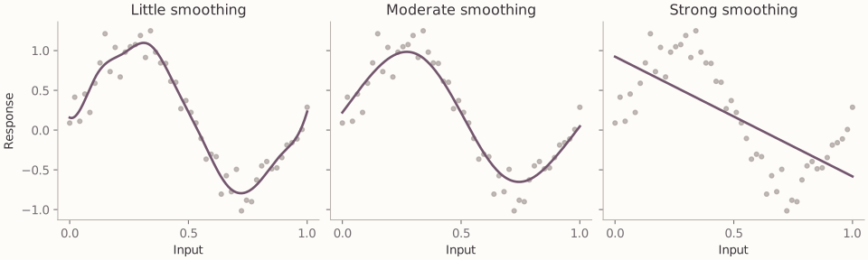
Three spline fits to the same simulated observations with increasing curvature penalties. — Illustrative simulated data with one fixed cubic basis. Increasing the curvature penalty moves the estimate toward a straight line. The observations and knots are identical in all three panels.

Separating penalized and unpenalized directions¶

Let $S=U_RDU_R^\top$ , where $D$ contains the positive eigenvalues, and let $U_F$ span its nullspace. Write

\beta=U_R\theta_R+U_F\theta_F.

(8)

Then

B\beta=BU_R\theta_R+BU_F\theta_F,\qquad\beta^\top S\beta=\theta_R^\top D\theta_R.

(9)

The $F$ component is a free linear trend. The $R$ component describes curvature and is penalized. Setting $\gamma=D^{1/2}\theta_R$ turns its penalty into $\lVert\gamma\rVert^2$ , with transformed design $BU_RD^{−1/2}$ . This makes the connection to ordinary ridge explicit.