Basic
Metrics
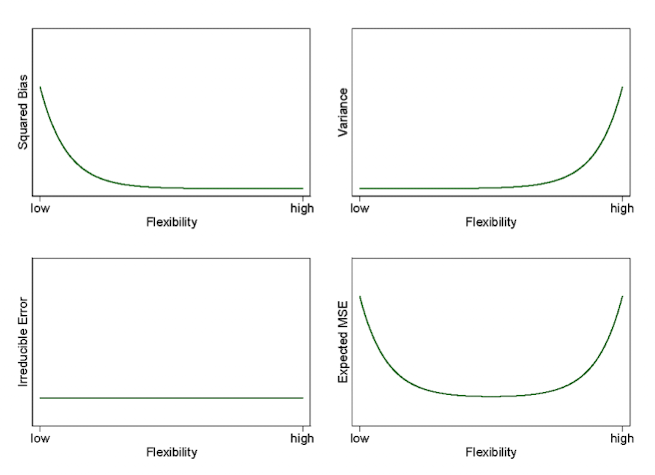
Expected MSE
For a continuous outcome, prediction error comes from systematic error, sensitivity to the training sample, and noise in the new outcome.
| Component | Meaning |
|---|---|
| Bias | How far the average fitted prediction is from the true function: . |
| Variance | How much the fitted prediction changes across new training samples. |
| Noise | Variation in a new outcome that remains even if the true function is known. |
We want both low bias and low variance. Irreducible noise sets a lower bound on prediction error.
What is being averaged?
Write , with . Hold fixed and refit the same method on new training samples. The fitted values change across those samples; the new observation also has its own noise.
The decomposition assumes that the new observation’s noise is independent of the training sample. If noise variance changes with , use . This is a squared-error result; classification error does not have the same decomposition.
Accuracy
| Predicted True | Predicted False | |
|---|---|---|
| Actual True | TP | FN |
| Actual False | FP | TN |
Used for Categorical problems.
Refers to the percentage of correctly identified observations.
Sensitivity and Specificity
Sensitivity
Share of actual positives correctly identified. Also called the true-positive rate or recall.
Its denominator includes all actual positives; missed positives reduce sensitivity.
We want high sensitivity and high specificity, but changing the classification threshold usually trades one against the other.
Multi-Class Classification
Precision/recall must be evaluated for each class when there are multiple classes.
Macroaveraging:
Each classes get equal weights during evaluation. By ignoring class size, gives rare categories the same weight as frequent categories.
E.g., Computing -values for each 2,2 classification table and averaging the -values afterwards.
Microaveraging:
Aggregate all predictions first, then compute the metric.
Sum all TP, FP, FN across classes.
Gives more weight to large classes.
Useful when we care about the overall accuracy, and when the data is imbalanced.
Compute the metric after pooling TP, FP, and FN; averaging class-specific scores instead would be macroaveraging.
E.g., Pooling all the 2,2 tables into a single 2,2 table and computing -values based on the pooled tbable.
ROC
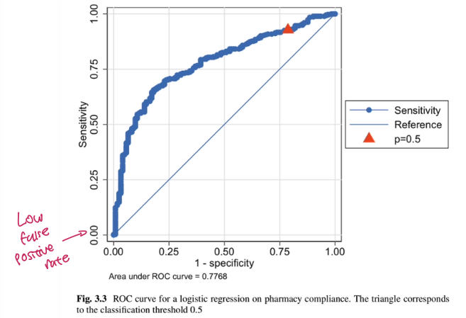
A receiver operating characteristic (ROC) curve shows how the true-positive and false-positive rates change as the classification threshold moves.
| Axis | What it measures |
|---|---|
| Horizontal | False-positive rate: , or . |
| Vertical | True-positive rate: , also called recall or sensitivity. |
Points near the upper-left corner combine high sensitivity with a low false-positive rate.
Constructing the curve
01 / Order
Sort observations by predicted probability of the positive class.
02 / Threshold
At each cutoff, classify observations at or above it as positive and those below it as negative.
03 / Plot
Calculate FPR and TPR at each cutoff, then plot the resulting points.
F-Measure
F₁ combines precision and recall. It does not reward correct negative predictions, so a large number of true negatives cannot inflate the score. Values range from 0 to 1, with higher values indicating a better precision–recall balance.
| Metric | Question |
|---|---|
| Precision | How many predicted positives are correct? . |
| Recall | How many actual positives are found? . |
Useful when
The positive class matters, and you need one summary of precision and recall. Examples include fraud detection and disease screening, where positives may be rare.
Check first
F₁ gives precision and recall equal importance. If false positives and false negatives have different costs, examine them separately and choose a threshold using those costs.
With balanced classes and symmetric error costs, accuracy may also be useful. RMSE applies to numerical prediction, rather than class labels. Emphasize precision to limit false positives, and recall to limit missed positives.
Choosing a threshold
If a false positive costs and a false negative costs , the expected costs at a point with probability are
This calculation needs probabilities that reflect the population where predictions will be used. A good AUC only establishes good ranking; it does not establish that a predicted probability of 0.8 is reliable.
Baseline
Bayes Classifier
A baseline model with an assumption that test errors are minimized when each new observation is assigned to the most likely class.
For a new observation, choose the class with the largest probability.
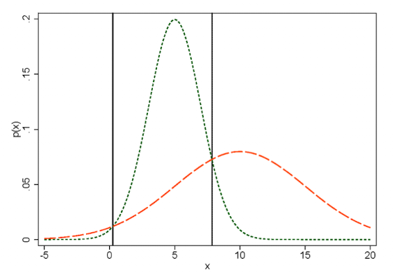
From the graph above, there are two noticeable boundaries where can lead to a change of membership to a new observation, one at 0 and the other at 8.
Error rate (For a given observation ):
Error rate (Overall Bayes error rate):
The Bayes error rate is the minimal error rate.
However, in practice, Bayes error rate is never known, because the underlying functions are not known.
Overfitting and Underfitting
Overfitting
Overfitting happens when the model fits random noise of a sample rather than the generalizable relationship.
When does it happen?
When the model has too many parameters relative to the number of observations.
This is why advanced machine learning algorithms must be watchful towards overfitting; they are designed to have a lot of parameters.
When the model is too flexible; when a model can fit a wide variety of shapes and patterns in the data.
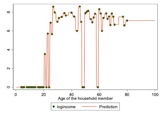
As can be seen on the graph above, overfitted model can twist and bend very closely on data.
Underfitting and validation
An underfitted model misses a pattern that is present in the data. Both training and validation errors can remain high. An overfitted model often has low training error but noticeably higher validation error. The gap is useful evidence, although different training and validation populations can also cause a gap.
Use the training set to estimate parameters and a validation set, or cross-validation within the training data, to choose model settings. Keep the test set for evaluating the chosen procedure. Trying many settings on the test set gradually makes it part of model selection.
In -fold cross-validation, each fold is held out once while the other folds are used for fitting. Preprocessing must also be fitted again within each training fold. For repeated measurements, keep observations from the same subject together. For future prediction, use splits that preserve time order.
Tips
Log Transformation
When or any variable spans multiple magintude, it is easier to take a log of it. (E.g., )
Log transformation reduces the scale of very large values more than small ones.
E.g.:
→
→
Hence, log transformations can shrink gaps dramatically, and prevent large values from dominating the model.
Can reduce right skewness of a positive variable and make some relationships easier to model; improvement is not guaranteed. A logarithm needs positive inputs, and back-transforming a prediction of log response does not generally give the mean response.
Nonlinear models
A model is nonlinear if parameters () appear nonlinearly, not the predictors (). For example,
... is nonlinear, because you cannot seperate and into a clean linear combination. For example, neural networks have their weights interacting across layers and are an example of nonlinear model.
| Example | Linear in coefficients? | |
|---|---|---|
| Linear regression | Yes | |
| Logistic regression | Yes (in log odds) | |
| Nonlinear model | No |
Linear Model
This model above is called as ordinary linear regression (OLR).
Least squares gives the best linear unbiased estimator under the Gauss–Markov assumptions: a correctly specified linear conditional mean, full column rank, and errors with zero conditional mean, constant variance, and no correlation.
AKA, has the lowest variance.
Refers to a specific way to esimate the coefficients .
Chooses by minimizing: .
Hyperparameter and Parameter
Parameter
A value estimated from training data when fitting the model.
Examples
Regression coefficients .
Weights in logistic regression and neural networks.
Hyperparameter
A setting that controls the model or fitting procedure. Choose it before an individual fit, often by comparing validation results across fits.
Examples
in -NN.
in ridge and LASSO regression.
max_depthin tree models.learning_ratein boosting.