Preprocessing

One-Hot Encoding¶

Use indicator variables or dummy variables and convert categorical variables into a numeric format that machine learning models can understand.
E.g., Suppose we have a variable with binary values, including “woman” and “man”.
- Create an indicator variable, $I_\text{male}$ .
- Then, $I_\text{female}$ = $1 - I_\text{male}$
- In the $X$ -matrix, the concept of the two indicators area collinear. Hence, $I_\text{male} + I_\text{female} = 1$ .
- One variable of the two should not be included to avoid collinearity.

Reference category¶

With an intercept and $K$ categories, use $K-1$ indicators in an unpenalized linear or logistic model. The omitted category becomes the reference. Its fitted value is represented by the intercept, and each indicator coefficient compares its category with that reference, holding the other predictors fixed.

E.g., With categories A, B, and C, use indicators for B and C. An observation in A has both indicators equal to 0. Keeping all three indicators as well as an intercept creates exact linear dependence because their sum is always 1. This is a statement about the design matrix; tree models do not require the same reference-category convention.

An integer code such as A=1, B=2, C=3 also introduces an order and spacing. Use it only if those properties make sense for the model. Decide how unseen categories will be handled before evaluating new data.

Variable Scaling¶

Standardization¶

z = \frac{x - \mu}{\sigma}

(1)

Centers data around 0 (mean = 0) and a unit standard deviation (standard deviation = 1).
Keeps the shape of distribution.
Values are not bounded.
When to use:
- Useful for most ML models.
- When comparable units are needed; standardization itself is not robust to outliers.
- When data distribution matters.
Indicator variables may or may not be scaled.

Scaling¶

Min-Max scaling.
$x = \frac{x-\text{min}}{\text{max} - \text{min}}$
(2)
Limits the data range within $[0,1]$ .
Does not affect indicator variables at all.
Rescales values into fixed range.
Preserves relative distances.
When to use:
- When you want bounded values.
- Neural networks.
- Image data.

Fit transformations on training data¶

The mean, standard deviation, minimum, and maximum are estimated from the training data. Apply those same values to validation and test observations. Otherwise, the transformation has already used information from the data reserved for evaluation.

E.g., If the training mean is 50 and standard deviation is 10, a new value of 70 becomes $(70-50)/10=2$ . Do not recompute the mean after adding the new observation. Similarly, a test value outside the training range can become less than 0 or greater than 1 after min–max scaling.

Standardization changes units, not distributional shape. A skewed variable remains skewed, and an extreme observation can strongly affect both the mean and standard deviation. Median and interquartile range provide a less outlier-sensitive alternative. A constant predictor has zero standard deviation and needs separate handling.

Missing values¶

A missing value is not automatically zero. For example, an unrecorded income and an income of zero describe different situations. Median imputation for a numerical variable and a separate missing category for a categorical variable are simple starting points. Estimate imputation values on training data only.

A missingness indicator can retain information about whether a value was observed. It does not explain why the value is missing or remove bias caused by the missingness process. The same missing-value rules must be available when a new observation arrives.

Text Preprocessing¶

Word Base Form¶

Stemming¶

Crude chopping of word endings.
Uses simple rules without understanding meaning of words.
Oftne produces non-real words.
Rule-based:
- Keep double $\text{ss}$ , such as chess.
- Replaces $\text{~ies}$ at the end with $\text{i}$ . E.g., parties → parti.

Lemmatization¶

Reduces words to their dictionary form (hence, lemma).
Uses vocabulary and grammar (POS tagging.)
Produces real words.
E.g., running → run, studies → study, better → good (Keep context).

TF-IDF¶

Stands for Term Frequency - Inverse Document Frequency.
Usually, TF-IDF is computed after stemming.

TF¶

\text{TF} = \begin{cases} 1 + \log(f_{t,d}) & \text{if } f_{t,d} > 0 \\ 0 & \text{otherwise} \end{cases}

(3)

$f_{t,d}$ = Number of times a term $t$ appears in document $d$ .
- E.g., If a word “enjoy” appears only once, then $1+\log{1} = 1$ . If appears 100 times, then $1+\log{100} = 5.6$ .

IDF¶

Rare words are more useful than frequently used words; rare words are given more weight.
Document means “text for one observation”, such as one movie review, one answer to an open-ended question.
$\text{IDF} = \log{\frac{N}{N_t}}$
(4)
$N$ = Sample size, $N_t$ = Number of documents containing term $t$ at least once.
This function decreases as a function of term frequency.
Together with TF, $\text{TF} \cdot \text{IDF}$ creates:
$((1+\log{f_{t,d}}) \times \log{\frac{N}{N_t}})$
(5)

Example

$N = 5$ (5 documents)
E.g., Computing the score for “sir”:
- “sir” appears in document 1, 2, 3, 5.
- Hence $N_t = 4$ .
IDF: $\log{\frac{N}{N_t}} = \log{\frac{5}{4}} = 0.223$ .
TF in the second document for example:
- “sir” appears twice in the second document. Hence, $1+\log{2} = 1.69$ .
  $\text{TF} \cdot \text{IDF} = 1.69 \times 0.223 = 0.38$
  (6)

Doc	quarrel	sir	no	better
1	0.916	0.223	0	0
2	0.916	0.378	0.223	0
3	0	0.223	0	0
4	0	0	0.223	0.916
5	0	0.223	0	0

TF-IDF creates document-term matrix just as Bag of Words, but containing values that are weights, not counts.
Used when:
- Want to reduce noise from common words.
- Highlights meaningful terms.
- Improves similarity comparisons.

Vocabulary and document frequency¶

The vocabulary fixes what each column means. Learn it from training documents and reuse the same columns for new documents. IDF is also learned from the training corpus; recomputing it on the test documents changes the representation used for evaluation.

The TF formula above uses a logarithm, whereas raw-count TF would use $f_{t,d}$ directly. These give different weights when a term occurs more than once. Here, the weight for “sir” in document 2 is $(1+\log 2)\log(5/4)\approx0.378$ . The choice of TF convention must stay the same throughout a calculation.

Stemming is optional. It can combine useful word variants, but it can also combine words that should stay distinct. Negation also needs care: removing “not” can change the meaning of “not good” completely.

Text Similarity¶

A value of 0 indicates that text documents are dissimiliar, and 1 indicates that the documents are functionally identical.

Cosine Similarity¶

\cos(\theta) = \frac{\bar{x}_1 \cdot \bar{x}_2}{\|\bar{x}_1\| \, \|\bar{x}_2\|}

(7)

Good representation of similarity between the vector representations of two text documents.
Used in nearnest neighbor algorithms, vector space model in information retrieval (e.g., searching for information on the web.)
$x_1$ and $x_2$ are the two text documents.

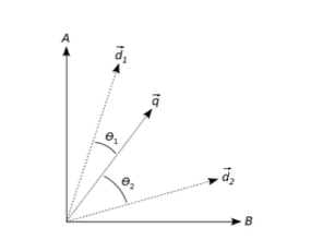
Assume $\bar{q}$ , $\bar{d}_i$ are documents.
From the diagram, document $q$ is closer to $d_1$ than $d_2$ . Return documents that have minimal angle to $q$ .
Cosine similarity of $1 = \text{Cos}(0) \text{ degrees}$ : Vectors heading towards exactly same direction.
Cosine similarity of $0 = \text{Cos}(90) \text{ degrees}$ : Vectors are orthogonal to one another.

Example

From the image above, we have two vectors:
- $x_1 = (2, 1, 1, 1, 0, 0, 0)$
- $x_2 = (2, 0, 0, 0, 1, 1, 1)$
Compute cosine similarity between two:
- $\cos(\theta) = \frac{\bar{x}_1 \cdot \bar{x}_2}{\|\bar{x}_1\| \, \|\bar{x}_2\|} = \frac{4}{\sqrt{7} \cdot \sqrt{7}} = 0.57$
- $\bar{x}_1 \cdot \bar{x}_2 = 4+0+0+0+0+0+0 = 4$
- $\|\bar{x_1}\| = \sqrt{\sum{x_1^2}} = \sqrt{2^2+1^2+1^2+1^2} = \sqrt{7}$
- Interpretation: The cosine of the angle is about 0.57; this is not the percentage of shared words.
Document lengths do not matter in cosine similarity.
Text order is not preserved in cosine similarity.

Usage

When you care about topic/content similarity
Document comparison/retrieval
High-dimensional sparse data
Length of documents shouldn’t matter

Limitations

Do NOT use when:
- Word order matters.
- When meaning of words are important (being able to recognize synonyms).
- When context matters. (“bank” for either “river bank” or “finance bank” is oblivious.)
- When sentence-level semantics matter (e.g., subtle meaning differences, tone, sentiment, intent.)

Jaccard Similarity¶

J(A, B) = \frac{|A \cap B|}{|A \cup B|}

(8)

$A \cap B$ = Elements in both.
$A \cup B$ = Elements in either.
Measures how much two sets of data overlap relative to their total size.
Ignores the words that are in neither of the two sets (True Negatives.)
Can also be written as:
$\text{Jaccard} = \frac{TP}{TP + FP + FN}$
(9)
And should mean the same as above.
TP: Elements in both sets. Hence, $TP = |A \cap B|$
FP: In A but not in B.
FN: In B but not in A. Hence, $TP + FP + FN = |A \cup B|$

Example

Set	Elements
A	apple, banana, orange
B	banana, orange, grape

Intersection: {banana, orange} = 2.
Union: {apple, banana, orange, grape} = 4.
- TP: {banana, orange} = 2
- FP: {apple} = 1
- FN: {grape} = 1
$J = \frac{2}{4} = 0.5$

Usage

Binary or set data (e.g., presence and absence of words in doucment, items in bucket.)
Duplicate detection.
- Near-duplictate documents.
- Plagiarism detection.
Sparse data that we are only intereseted in shared items.

Limitations

When frequency matters. Jaccard ignores counts.
- E.g., “Word appears 10 times vs. 1 time” is the same in Jaccard.
When using TF-IDF.
- Jaccard is set for sets, not weighted vectors.
When meaning matters.
- Cannot capture synonyms, context, order.

Feature	Jaccard	Cosine
Uses counts	No	Yes
Uses weights	No	Yes
Based on	set overlap	vector angle

For cosine similarity, multiplying either nonzero vector by a positive constant leaves the angle unchanged. A score of 1 therefore means the vectors have the same direction, not necessarily the same word counts. With nonnegative term vectors, cosine lies between 0 and 1; for general signed vectors it can be negative. An all-zero vector has no defined cosine similarity.

Jaccard answers a different question: how much of the combined set is shared? It ignores repeated occurrences, so repeating every word in one document changes neither its set nor its Jaccard similarity. Choose the representation before interpreting the score.

Levenshtein Distance¶

Measures how many single-character edits are needed to turn one string into another.
Costs 1 for every operation of:
- Inserting a character
- Deleting a character
- Substituting (replacing) a character
E.g., Transforming “Kitten” into “Sitting”.
- Substitude “S” in place of the first “K” (1)
- Substitute “i” iu place of “e” (1)
- Inserting “g” at the end (1)
- Hence total Levenshtein Distance is: $1+1+1=3$ .

BM25¶

A probabilistic ranking function used in information retrieval to score and rank documents based on their relevance to a search query.

Improves TF-IDF by:
1. Term frequency saturation: After a word appears several times in a document, additional occurrences matter less. (Diminishing returns.)
2. Document length normalization: Longer documents naturally contain more term matches, and BM25 adjusts this.

\text{BM25}(D, Q) = \sum_{i=1}^{n} \text{IDF}(q_i) \cdot \frac{f(q_i, D) \cdot (k_1 + 1)}{f(q_i, D) + k_1 \cdot \left(1 - b + b \cdot \frac{|D|}{\text{avgdl}}\right)}

(10)

\text{IDF}(q_i) = \ln\left(\frac{N - n(q_i) + 0.5}{n(q_i) + 0.5} + 1\right)

(11)

Variable	Meaning
$f(q_i, D)$	Term frequency of $q_i$ in document $D$
$\lvert D \rvert$	Length of document $D$ in words
$\text{avgdl}$	Average document length across the corpus
$N$	Total number of documents in the corpus
$n(q_i)$	Number of documents containing the term $q_i$
$k_1$	Term frequency saturation parameter (typically $1.2 \leq k_1 \leq 2.0$ )
$b$	Length normalization parameter (typically $b = 0.75$ )

Solutions Key

One-Hot Encoding¶

Reference category¶

Variable Scaling¶

Standardization¶

Scaling¶

Fit transformations on training data¶

Missing values¶

Text Preprocessing¶

Word Base Form¶

Stemming¶

Lemmatization¶

TF-IDF¶

TF¶

IDF¶

Vocabulary and document frequency¶

Text Similarity¶

Cosine Similarity¶

Jaccard Similarity¶

Levenshtein Distance¶

BM25¶

1. Term Frequency with Saturation (TF)¶

2. Inverse Document Frequency (IDF)¶

3. Document Length Normalization¶

4. Score Aggregation¶