Regression Trees
A regression tree predicts a numerical response by asking a sequence of questions about the predictors. Each observation follows one path to a terminal region, or leaf, and receives the fitted value assigned to that region.
Interactions without a full expansion
In the model , increasing by one changes the fitted mean by . The effect depends on , which is the meaning of an interaction.
With predictors, including one product for every subset gives terms including the intercept. There are interactions involving at least two distinct predictors. This count concerns products with each variable appearing at most once; allowing arbitrary powers creates a different expansion.
A tree can express conditional behavior by splitting on one predictor only after a condition on another has been met. It does not require us to enumerate every possible product in advance.
A partition model
Let be disjoint regions covering the input space. Then
Exactly one indicator is one for each input, so the prediction is the constant of its leaf. A fixed collection of regions would give a linear basis model. An estimated tree is different because the regions themselves are chosen using the responses.
Why a leaf predicts its mean
For a fixed nonempty region , minimize . Its derivative is
giving . This is specific to squared error; other losses can imply different leaf predictions.
For an illustrative leaf with responses , the prediction is 4 and the residual sum of squares is . Splitting it into responses and gives means 2.5 and 7, with total residual sum of squares 0.5. The training improvement is 13.5, although prediction improvement still needs validation.
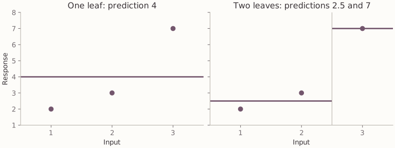
Illustrative inputs 1, 2, and 3 paired with responses 2, 3, and 7. A threshold at 2.5 reduces training RSS from 14 to 0.5. This demonstrates a training improvement, not evidence of improved future prediction.
Choosing a split
Within a node , a candidate feature and threshold produce
For a numerical feature, only boundaries between distinct sorted observed values need examination. Every threshold inside such a gap gives the same allocation of training observations. Enforce any minimum node size before comparing candidates.
Repeat this search inside the resulting nodes. This procedure is greedy: it chooses the best immediate split, not the globally best complete tree. Ties can occur, and small changes to the sample can change an early split and all branches below it.
Pruning
A large initial tree can fit noise. For a subtree , let denote its number of leaves and define
The first term rewards fit; the second charges for leaves. In the lecture notation, is the residual sum of squares in leaf , so summing it over leaves gives the same RSS.
Pruning replaces a branch by a single leaf. Its RSS increases, but its complexity charge decreases. In the numerical example above, replacing one leaf by two reduces RSS by 13.5 and adds one leaf. This local comparison favors keeping the split when , with a tie at 13.5.
In a complete tree, compare candidate subtrees along a pruning sequence. Select complexity using validation predictions, then assess the selected procedure separately. The smallest training RSS always favors a sufficiently large tree and is not a tuning criterion by itself.
Usage
Relationships contain thresholds or conditional interactions.
A short sequence of decision rules is useful for explanation.
A flexible model is needed without a prespecified polynomial expansion.
Limitations
Small sample changes can produce different splits.
Predictions are piecewise constant and can be discontinuous.
A single tree can have high variance.
Leaf means do not extrapolate a rising or falling trend beyond the observed responses.
The classification tree notes use the same partition idea with a categorical response. The response type changes the loss, splitting criterion, and leaf prediction.