Solution Paths and Selection - The Statistics Notebook

A solution path records how the fitted coefficients change as the penalty varies. It makes fitting many candidate models efficient, but it does not tell us which candidate predicts best. Validation supplies that separate decision.

Starting from the zero slope model¶

With centered data and $\beta=0$ , the residual is $y$ . The zero vector satisfies the LASSO optimality conditions exactly when $|x_j^\top y|\leq\lambda$ for every $j$ . Therefore,

\lambda_{\max}=\max_j|x_j^\top y|.

(1)

Every penalty at least this large has zero as an optimal slope vector. An unpenalized intercept remains at the training mean. Under a mean loss convention, the threshold is divided by $n$ .

Warm starts¶

Choose a decreasing sequence beginning at $\lambda_{\max}$ . Solve the first problem, then use its coefficients as the starting point for the next penalty. Neighboring problems often have similar solutions, so this avoids repeatedly starting far from the answer.

Warm starts are computational devices. Each candidate must still converge to the required tolerance. They do not replace validation and do not establish that coefficients enter in a fixed ranking of their original correlations with the response.

Why the path is piecewise linear¶

Suppose the active set $A$ and its sign vector $s_A$ remain fixed over a penalty interval, and $X_A$ has full column rank. The active optimality equations are

X_A^\top(y−X_A\beta_A)=\lambda s_A.

(2)

Rearranging,

\beta_A(\lambda)=(X_A^\top X_A)^{−1}X_A^\top y−\lambda(X_A^\top X_A)^{−1}s_A.

(3)

Within this interval, the coefficients are affine functions of $\lambda$ . A segment ends when an active coefficient reaches zero or an inactive variable reaches its residual correlation threshold. The set and signs can then change.

A coefficient may leave and later reenter. The number of selected variables is not guaranteed to increase at every step as the penalty decreases. Degenerate designs also require care in choosing among coefficient solutions; the displayed inverse assumes an independent active design.

Reading a coefficient plot¶

A flat zero segment identifies penalties where a coefficient is absent. A change in slope marks a change in the active configuration. Correlated columns can alter one another’s coefficient paths without any statistical interaction term being present.

Piecewise linearity is with respect to $\lambda$ itself. If the horizontal axis is $\log\lambda$ , a straight segment in $\lambda$ will generally appear curved. Axis labels matter when comparing the derivation with a software plot.

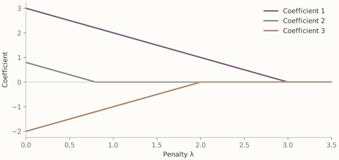
Three orthogonal LASSO coefficients shrink to zero at penalties 0.8, 2, and 3. — Exact paths for the orthogonal example with correlations 3, 0.8, and −2. The horizontal axis is the penalty itself. Each path is linear until it reaches zero; correlated designs can have more complicated active set changes.

Choosing the penalty¶

For each candidate penalty, fit the entire procedure on the training portion of each fold and predict its validation portion. Average the validation loss. For numerical responses, squared error is a common choice.

The minimum error rule selects the penalty with the smallest estimated validation error. The one standard error rule selects the largest penalty whose estimated error is no more than the minimum error plus the estimated standard error at that minimum. It favors a more strongly penalized model when the estimated differences are small.

This is a model selection rule, not a 95 percent confidence interval or a test proving equal predictive performance. Fold errors are dependent, and the reported standard error is an approximation to uncertainty in the validation curve.

After choosing a model¶

Refit using all designated training data with the selected penalty and training preprocessing. Evaluate on the reserved test data, or use an outer validation loop to assess the complete selection process.

Compare stability as well as average error when interpretation matters. If different folds select different members of a highly correlated group, it is more accurate to report that uncertainty than to treat one final active set as uniquely established.