Factorial Experiments & Interaction - The Statistics Notebook

A factorial experiment studies combinations of two or more design factors. It asks how each factor changes the response and whether its effect depends on another factor.

This extends One-Way ANOVA: a second factor can be a scientific treatment factor, rather than merely a nuisance variable to remove.

Design	Treatment combinations	Main question
Two factors with $a$ and $b$ levels	$ab$	What are the effects of A, B, and their interaction?
Three factors with $a,b,c$ levels	$abc$	Does a two-factor interaction depend on the third factor?
$k$ factors, each with two levels	$2^k$	Which factors and interactions are active over the chosen ranges?

With $n$ independent replicates per combination, multiply the number of combinations by $n$ to obtain the total run count. All raw numerical data used below are illustrative.

Why Vary Factors Together?¶

Suppose A is a process setting and B is a temperature setting. Changing A only at low B tells us its effect at low B. It cannot show whether A behaves differently at high B.

A factorial design includes every combination, allowing us to estimate both main effects and interactions. Each run contributes to several comparisons. The cost is that the run count grows as the product of the numbers of levels.

Choose factors and ranges with a scientific purpose. A low/high difference that is too small may be practically uninformative; a very wide range can make a simple model inappropriate. Randomize execution order and use independent experimental units.

Main Effects, Simple Effects & Interaction¶

Quantity	Meaning
Simple effect of A	Change in mean response across A levels at a particular level of B.
Main effect of A	A comparison averaged over B levels, using the stated weighting.
Interaction	The simple effect of A changes with B; equivalently, B’s effect changes with A.

For a balanced two-by-two design, let $\mu_{ij}$ denote the mean at A level $i$ and B level $j$ . The simple effects of increasing A are

\Delta_A(B_1)=\mu_{21}-\mu_{11},\qquad \Delta_A(B_2)=\mu_{22}-\mu_{12}.

(1)

Their difference is the difference of differences:

D_{AB}=(\mu_{22}-\mu_{12})-(\mu_{21}-\mu_{11}).

(2)

No interaction means $D_{AB}=0$ . In an interaction plot, parallel population-mean lines indicate additivity. Sample lines need not be perfectly parallel even when the population model is additive.

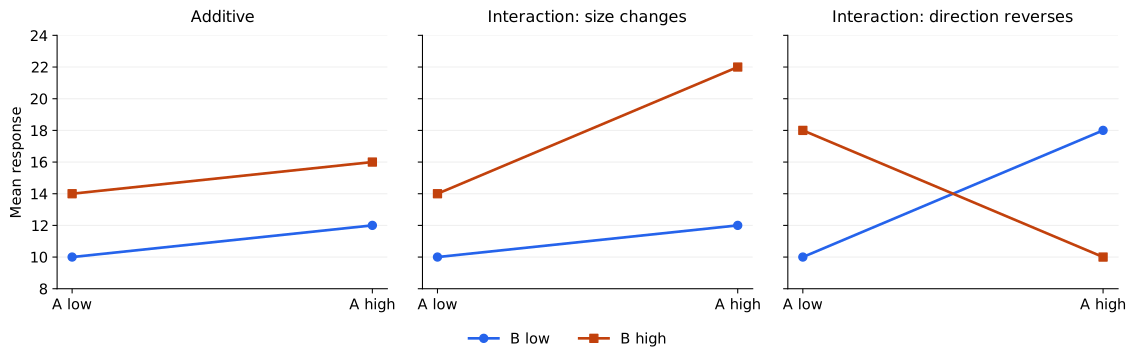
Additive, changing-size, and crossover interaction patterns.

Nonparallel lines need not cross to indicate interaction. A crossover can make an average main effect near zero even when the factor matters greatly within each condition. A plot suggests patterns; inferential uncertainty still matters.

Worked Example: An Average Effect Hides Two Different Effects

Consider cell means:

	B low	B high	A marginal mean
A low	10	14	12
A high	12	22	17
B marginal mean	11	18	14.5 overall

The simple effect of A is $12-10=2$ at low B and $22-14=8$ at high B. The average high-minus-low effect of A is

17-12=5=\frac{2+8}{2}.

(3)

The difference of differences is $8-2=6$ . Reporting only “A raises the response by 5” would hide the dependence on B.

The largest observed mean is at high A, high B. That identifies the best observed combination if larger is better, not a proven global optimum or a guarantee for future observations.

Replicated Two-Factor Model¶

For A levels $i=1,\ldots,a$ , B levels $j=1,\ldots,b$ , and independent replicates $r=1,\ldots,n$ ,

Y_{ijr}=\mu+\alpha_i+\beta_j+(\alpha\beta)_{ij}+\varepsilon_{ijr},

(4)

\varepsilon_{ijr}\overset{\mathrm{iid}}{\sim}N(0,\sigma^2).

(5)

The usual constraints are

\sum_i\alpha_i=0,\qquad\sum_j\beta_j=0,

(6)

\sum_i(\alpha\beta)_{ij}=0\ \text{for each }j,\qquad \sum_j(\alpha\beta)_{ij}=0\ \text{for each }i.

(7)

These constraints make the parameterization identifiable. The cell mean is

\mu_{ij}=\mu+\alpha_i+\beta_j+(\alpha\beta)_{ij}.

(8)

Sample mean	Average over
$\bar Y_{ij\cdot}$	Replicates in cell $(i,j)$ .
$\bar Y_{i\cdot\cdot}$	All B levels and replicates at A level $i$ .
$\bar Y_{\cdot j\cdot}$	All A levels and replicates at B level $j$ .
$\bar Y_{\cdot\cdot\cdot}$	All $N=abn$ observations.

For this balanced design,

\widehat\mu=\bar Y_{\cdot\cdot\cdot},\quad \widehat\alpha_i=\bar Y_{i\cdot\cdot}-\bar Y_{\cdot\cdot\cdot},\quad \widehat\beta_j=\bar Y_{\cdot j\cdot}-\bar Y_{\cdot\cdot\cdot},

(9)

\widehat{(\alpha\beta)}_{ij} =\bar Y_{ij\cdot}-\bar Y_{i\cdot\cdot}-\bar Y_{\cdot j\cdot}+\bar Y_{\cdot\cdot\cdot}.

(10)

Thus $\widehat Y_{ijr}=\bar Y_{ij\cdot}$ and $e_{ijr}=Y_{ijr}-\bar Y_{ij\cdot}$ . The interaction is the cell mean’s departure from what the additive main-effects model predicts.

Two-Factor ANOVA¶

For equal replication, variation splits into four orthogonal components:

SS_T=SS_A+SS_B+SS_{AB}+SS_E.

(11)

\begin{aligned} SS_A&=bn\sum_i(\bar Y_{i\cdot\cdot}-\bar Y_{\cdot\cdot\cdot})^2,\\ SS_B&=an\sum_j(\bar Y_{\cdot j\cdot}-\bar Y_{\cdot\cdot\cdot})^2,\\ SS_{AB}&=n\sum_{i,j}\left(\bar Y_{ij\cdot}-\bar Y_{i\cdot\cdot}-\bar Y_{\cdot j\cdot}+\bar Y_{\cdot\cdot\cdot}\right)^2,\\ SS_E&=\sum_{i,j,r}(Y_{ijr}-\bar Y_{ij\cdot})^2. \end{aligned}

(12)

Source	df	Mean square	Test
A	$a-1$	$MS_A=SS_A/(a-1)$	$F_A=MS_A/MSE$
B	$b-1$	$MS_B=SS_B/(b-1)$	$F_B=MS_B/MSE$
AB	$(a-1)(b-1)$	$MS_{AB}=SS_{AB}/[(a-1)(b-1)]$	$F_{AB}=MS_{AB}/MSE$
Error	$ab(n-1)$	$MSE=SS_E/[ab(n-1)]$
Total	$abn-1$

Each test uses its row’s df in the numerator and the error df in the denominator, with right-tail rejection. The hypotheses are all A effects zero, all B effects zero, and all interaction effects zero, respectively. With interactions present, main-effect hypotheses concern marginal averages, not absence of every simple effect.

These simple SS formulas rely on balance. For unequal replication or missing cells, fit the appropriate linear model and specify the desired comparisons and weighting; different adjusted ANOVA hypotheses need not coincide.

Worked ANOVA with Independent Replication

Use three observations per cell:

	B low	B high
A low	9, 10, 11	13, 14, 15
A high	11, 12, 13	21, 22, 23

Each cell has within-cell SS equal to 2, so $SS_E=8$ , error df $=4(3-1)=8$ , and $MSE=1$ .

The marginal means are A: $(12,17)$ and B: $(11,18)$ , with grand mean 14.5. Therefore,

SS_A=6[(12-14.5)^2+(17-14.5)^2]=75,

(13)

SS_B=6[(11-14.5)^2+(18-14.5)^2]=147.

(14)

The estimated interaction deviations are

\begin{pmatrix}1.5&-1.5\\-1.5&1.5\end{pmatrix},

(15)

so $SS_{AB}=3(4)(1.5^2)=27$ .

Source	SS	df	MS	$F$
A	75	1	75	75
B	147	1	147	147
AB	27	1	27	27
Error	8	8	1
Total	257	11

The interaction test is $F_{AB}=27$ on $(1,8)$ df. Interpret the simple effects of A, 2 and 8, to explain this interaction. All three tests are individually significant at 5% in this illustrative example; family-wide claims need an appropriate multiplicity plan.

Interpreting & Checking the Model¶

Inspect cell means and interaction plots. Begin interpretation with the highest-order interaction retained in the model.
Describe relevant simple effects when averages hide important differences.
Use planned contrasts or adjusted comparisons when several conclusions are intended jointly.
Check residual normality, spread across cells, outliers, and patterns over run order. Independence comes from the assignment and measurement design.
Report effects in response units, uncertainty, and the combinations actually studied.

Model hierarchy: retain the main effects A and B when retaining AB, even if one marginal test is nonsignificant. A nonsignificant interaction is not proof of additivity, especially with little replication.

Reference-group coding, sum-to-zero coding, and a separate parameter for each cell describe the same full cell-means model. Fitted values and residuals agree; coefficients have different interpretations. In reference coding, the intercept can be a baseline cell mean rather than the grand mean.

What Changes Without Replication?¶

With one observation per cell, $N=ab$ . The full interaction model fits every cell exactly and leaves zero pure-error df. Interaction can be described from cell values, but it cannot be tested against a separately estimated within-cell error variance from those data alone.

If additivity is scientifically defensible, fit

Y_{ij}=\mu+\alpha_i+\beta_j+\varepsilon_{ij}.

(16)

The fitted value is $\bar Y_{i\cdot}+\bar Y_{\cdot j}-\bar Y_{\cdot\cdot}$ . The remaining $(a-1)(b-1)$ df can serve as residual error under the no-interaction assumption. Any actual interaction is then mixed into that residual.

One observation per cell	What can be done?
Fit all cell means / full interaction	Estimate cell means; no internal pure-error estimate.
Fit an additive model	Test main effects conditionally on additivity and the error assumptions.
Obtain genuine replication or external error information	Supply information needed to separate interaction from noise.

Do not declare an interaction absent simply because a design cannot test it.

Quantitative Factors: Polynomial Components¶

For three equally spaced numerical levels, use linear coefficients $L=(-1,0,1)$ and quadratic coefficients $Q=(1,-2,1)$ . Each factor’s two df split into one linear and one quadratic component.

For A, with $bn$ observations contributing to each marginal mean,

C_A=\sum_i u_i\mu_{i\cdot},\qquad \operatorname{SE}(\widehat C_A)=\sqrt{\frac{MSE}{bn}\sum_i u_i^2}.

(17)

For an interaction component, take an outer product of contrast coefficients:

C_{uv}=\sum_{i,j}u_i v_j\mu_{ij},\qquad \operatorname{SE}(\widehat C_{uv})=\sqrt{\frac{MSE}{n}\left(\sum_i u_i^2\right)\left(\sum_j v_j^2\right)}.

(18)

For example, A-linear × B-quadratic uses

LQ^\mathsf T=\begin{pmatrix}-1&2&-1\\0&0&0\\1&-2&1\end{pmatrix}.

(19)

The four interaction components $L\times L$ , $L\times Q$ , $Q\times L$ , and $Q\times Q$ partition the four interaction df in the balanced $3\times3$ design. Each can be tested as a one-df contrast using the common MSE; adjust for multiplicity when making joint claims.

Polynomial contrasts require quantitative levels. The displayed coefficients assume equal spacing and balanced replication; arbitrary category labels do not have a linear or quadratic trend.

When Replicate Groups Are Blocks¶

If each complete factorial replicate was run in a different batch or week, the replicate index may represent a nuisance block. With $r$ complete blocks, one observation per treatment combination in each block, use

Y_{ij\ell}=\mu+\alpha_i+\beta_j+(\alpha\beta)_{ij}+\gamma_\ell+\varepsilon_{ij\ell}.

(20)

The balanced decomposition adds block SS with $r-1$ df. The residual df becomes

abr-1-(ab-1)-(r-1)=(ab-1)(r-1).

(21)

For a $3\times3$ factorial in two complete blocks, residual df is 8, compared with 9 when the two replicates are treated as unstructured replication. The treatment SS remain unchanged in this balanced orthogonal layout; MSE changes.

This model assumes treatment-block interactions are negligible. Without replication within each treatment-block cell, general treatment-block interactions cannot be separated from pure error. Design the blocking and randomization before collecting data.

More Than Two Factors¶

With three design factors, the full model includes A, B, C, AB, AC, BC, and ABC. An ABC interaction means that the AB interaction changes across C levels.

Term	df
A, B, C	$a-1$ , $b-1$ , $c-1$
AB, AC, BC	$(a-1)(b-1)$ , $(a-1)(c-1)$ , $(b-1)(c-1)$
ABC	$(a-1)(b-1)(c-1)$
Error with $n$ replicates per cell	$abc(n-1)$

The model’s non-intercept df sum to $abc-1$ . With $n=1$ , all df are consumed: more factors do not remove the need for replication or justified error assumptions.