Center Points & Curvature

A two-level factorial measures the corners of a region. Adding repeated runs at the center supplies information about reproducibility and whether the average corner response differs from the center response.

Center points detect a particular departure from the corner model. They do not identify a complete quadratic response surface.

Where Is the Center?¶

For a numerical factor with low and high settings $X_L,X_H$ ,

X_C=(X_L+X_H)/2,\qquad x_C=0.

(1)

With $k$ numerical factors, a center run sets every factor to its midpoint: $(0,\ldots,0)$ in coded units. Repeated center runs are separate experimental runs at the same design location.

Symbol	Meaning
$k$	Number of numerical factors in the basic setting.
$r$	Replicates per factorial corner.
$n_F=r2^k$	Total number of factorial observations.
$n_C$	Total number of repeated center observations.
$\bar Y_F$	Mean of all factorial observations, with equal replication per corner.
$\bar Y_C$	Mean of center observations.

Choose factor ranges so the midpoint is useful. It may represent the current operating condition, making center runs a check on familiar performance as well as curvature.

Spread center runs throughout the experiment. Interspersing them among the randomized factorial runs helps reveal drift. Running all centers at the end would mix location differences with time differences. Repeated measurements of one unchanged unit are not automatically independent center runs.

Categorical Factors Have No Midpoint¶

A factor coded $-1,+1$ may still be categorical. “Halfway between supplier A and supplier B” is not a valid setting.

Keep numerical factors at their midpoints and choose actual categorical levels. To examine curvature across all combinations of $q$ two-level categorical factors, there are $2^q$ possible center settings for the numerical factors.

Factors	Center settings for the numerical factors
A and B numerical	One: $(0,0)$ .
A numerical, B categorical	Two: $(0,B_1)$ and $(0,B_2)$ .
A, B numerical, C categorical	Two: $(0,0,C_1)$ and $(0,0,C_2)$ .
A numerical, B and C categorical	Four: numerical midpoint at each B-C combination.

The formulas below describe the basic all-numerical, balanced-corner case. With categorical factors, compare appropriate center and corner groups within categorical settings or use a model with the relevant terms. Pooling across categories can conceal different curvature patterns.

Why Compare the Corner Mean with the Center Mean?¶

A model with only an intercept and factor products is multilinear: no individual factor is squared. Every non-intercept product column averages to zero across a balanced full factorial, and every such term is zero at the all-zero center. Thus this model predicts the same average corner response and center response, even if interactions are present.

To interpret curvature locally, consider a second-order mean model:

\mu(\mathbf x)=\beta_0+\sum_{j=1}^k\beta_jx_j +\sum_{j<\ell}\beta_{j\ell}x_jx_\ell +\sum_{j=1}^k\beta_{jj}x_j^2.

(2)

At the center, all $x_j=0$ , so

\mu_C=\beta_0.

(3)

Across the balanced corners, the linear and cross-product terms cancel, while every $x_j^2=1$ . Therefore,

\mu_F=\beta_0+\sum_{j=1}^k\beta_{jj},\qquad \mu_F-\mu_C=\sum_{j=1}^k\beta_{jj}.

(4)

The curvature contrast tests

H_0:\mu_F-\mu_C=0,

(5)

which, under the second-order model, is equivalent to

H_0:\sum_j\beta_{jj}=0.

(6)

It does not test that every quadratic coefficient is individually zero. More complicated higher-order terms can also affect the corner-center contrast, so the quadratic interpretation is conditional on the assumed mean model.

Estimating Pure Error at the Center¶

Independent center runs have the same treatment setting. Their within-setting variation estimates error without needing a model for how the mean changes across factor settings:

s_C^2=\frac{\sum_{j=1}^{n_C}(Y_{Cj}-\bar Y_C)^2}{n_C-1}.

(7)

Its df is $n_C-1$ . At least two center replicates are needed for this estimate, and very few replicates make it imprecise.

This variance may be used for the whole experiment only when the common-variance and independence assumptions are appropriate. Center replication cannot demonstrate that corner variability is the same as center variability.

Deriving the Curvature Test¶

Assume independent normal errors with common variance $\sigma^2$ . Even though individual corner means may differ, their balanced average has variance $\sigma^2/n_F$ :

\operatorname{Var}(\bar Y_F-\bar Y_C) =\sigma^2\left(\frac1{n_F}+\frac1{n_C}\right).

(8)

With the center-only variance estimate,

T_{\mathrm{curv}}= \frac{\bar Y_F-\bar Y_C} {\sqrt{s_C^2(1/n_F+1/n_C)}}\sim t_{n_C-1}\quad\text{under }H_0.

(9)

Normality makes the center mean independent of its within-center variance; the factorial runs are independent of the center runs. These facts justify the $t$ reference distribution.

For a two-sided test, compare $|t|$ to $t_{1-\alpha/2,n_C-1}$ or compute its two-sided tail probability. A confidence interval for the contrast $\mu_F-\mu_C$ is

\bar Y_F-\bar Y_C\ \pm\ t_{1-\alpha/2,n_C-1} \sqrt{s_C^2(1/n_F+1/n_C)}.

(10)

Equivalent One-df $F$ Test¶

Using $1/n_F+1/n_C=(n_F+n_C)/(n_Fn_C)$ , define

SS_{\mathrm{curv}}=\frac{n_Fn_C}{n_F+n_C}(\bar Y_F-\bar Y_C)^2.

(11)

Then

F_{\mathrm{curv}}=\frac{SS_{\mathrm{curv}}/1}{s_C^2}=T_{\mathrm{curv}}^2 \sim F_{1,n_C-1}.

(12)

This numerator is sometimes called pure-quadratic SS. It has one df, regardless of the number of numerical factors. The error denominator has $n_C-1$ df when based only on center replicates.

Worked Curvature Example

Suppose eight factorial observations have mean $\bar y_F=71.25$ , and four independent center runs give $70,68,72,69$ .

\bar y_C=69.75,\qquad SS_{E,C}=8.75,\qquad s_C^2=8.75/3=2.9167.

(13)

The observed corner-center difference is 1.5. Its SE is

\sqrt{\frac{8.75}{3}\left(\frac18+\frac14\right)} =\sqrt{1.09375}=1.0458.

(14)

Thus

t=1.4343\quad(df=3),

(15)

SS_{\mathrm{curv}}=\frac{8(4)}{12}(1.5)^2=6,

(16)

F=\frac6{8.75/3}=2.0571=t^2.

(17)

The two-sided $t$ test and right-tail $F$ test give the same $p$ -value, approximately 0.2470. At 5%, this is insufficient evidence against a zero corner-center contrast.

The 95% interval is approximately $1.5\pm3.1824(1.0458)$ , or $(-1.83,4.83)$ . The uncertainty is substantial: this result does not prove that curvature is absent.

If Corners Are Replicated Too¶

If each of the $2^k$ corners has $r$ independent replicates, estimate pure error from within-corner and within-center variation together:

SS_{PE}=\sum_{i=1}^{2^k}\sum_{j=1}^r(Y_{ij}-\bar Y_i)^2 +\sum_{j=1}^{n_C}(Y_{Cj}-\bar Y_C)^2,

(18)

\nu_{PE}=2^k(r-1)+(n_C-1),\qquad MSE_{PE}=SS_{PE}/\nu_{PE}.

(19)

Under common variance, use this pooled MSE in the same curvature statistic, with $t_{\nu_{PE}}$ or $F_{1,\nu_{PE}}$ .

With all factorial effects included, the balanced augmented design has the decomposition

Component	df
Factorial effects among corners	$2^k-1$
Corner-center contrast	1
Pure error	$2^k(r-1)+n_C-1$
Total	$r2^k+n_C-1$

The contrast accounts for one mean difference; within-center SS accounts for variation around the center mean. Do not combine them into one error term when trying to test curvature.

What Center Points Cannot Identify¶

At every factorial corner, $x_1^2=\cdots=x_k^2=1$ . At the center, all these columns are zero. The pure-quadratic columns are therefore identical on this design.

Adding a center distinguishes their common column from the intercept, allowing estimation of their sum, but it does not separate the individual coefficients $\beta_{11},\ldots,\beta_{kk}$ .

A bowl has a nonzero corner-center difference, while a saddle can have curvature whose contributions cancel in the comparison.

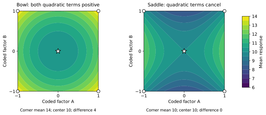
“Failure to detect curvature” means the particular contrast is not convincingly different from zero at the available precision. It does not establish linearity, rule out cancelling curvature, or validate extrapolation outside the experimental region.

Planning the Next Step¶

Finding	Interpretation	Useful follow-up
Detectable corner-center difference	The multilinear corner model misses a feature of the mean response.	Add design locations suitable for a quadratic or richer model.
No detectable difference, wide interval	Curvature contrast is poorly estimated.	Increase independent information if the uncertainty matters.
No detectable difference, narrow interval	That contrast is small within the interval.	Still consider cancellation and the intended prediction region.
Center responses drift over time	Process stability or run-order effects may be present.	Investigate conditions; account for relevant time or block structure.
Different scatter at corners and center	Common error variance is questionable.	Use an analysis and further replication that address heteroscedasticity.

Where Is the Center?¶

Categorical Factors Have No Midpoint¶

Why Compare the Corner Mean with the Center Mean?¶

Estimating Pure Error at the Center¶

Deriving the Curvature Test¶

Equivalent One-df FFF Test¶

If Corners Are Replicated Too¶

What Center Points Cannot Identify¶

Planning the Next Step¶

Equivalent One-df $F$ Test¶