Response Surfaces & Steepest Ascent - The Statistics Notebook

Response surface methodology is a sequential approach to improving a process with quantitative factors. Start with a local model, take informative steps, then redesign the experiment around the promising region.

A fitted plane gives a direction of improvement, not a finite unconstrained optimum. New observations are needed as the process moves beyond the initial experimental region.

The Sequential Strategy¶

Stage	Purpose
Local experiment	Estimate a first-order response model in a feasible starting region.
Directional runs	Move along a promising path and observe whether the response improves.
New local experiment	Recenter and investigate the shape near a promising region.
Optimization and confirmation	Fit a suitable richer model, identify a feasible candidate, and validate it with new runs.

This approach is especially useful after screening has reduced the number of active numerical factors. Categorical choices need separate comparisons or an appropriate mixed-factor design; they do not have a continuous direction to move along.

Coding & Decoding¶

For natural-unit factor $Z_j$ , center $c_j$ , and half-range $h_j>0$ ,

x_j=\frac{Z_j-c_j}{h_j},\qquad Z_j=c_j+h_jx_j.

(1)

Coding expresses changes relative to meaningful experimental ranges. It also defines the scale on which “steepest” is measured.

For A ranging from 30 to 40 and B from 150 to 160,

x_1=\frac{A-35}{5},\qquad x_2=\frac{B-155}{5}.

(2)

The center is $(35,155)$ , and both half-ranges are 5.

First-Order Model & Gradient¶

Fit a local first-order model

\widehat y(\mathbf x)=\widehat\beta_0+\sum_{j=1}^k\widehat\beta_jx_j =\widehat\beta_0+\mathbf b^\mathsf T\mathbf x.

(3)

Its gradient in coded units is $\mathbf b=(\widehat\beta_1,\ldots,\widehat\beta_k)^\mathsf T$ .

For a coded step of fixed Euclidean length $s$ , Cauchy-Schwarz gives

\mathbf b^\mathsf T\Delta\mathbf x\leq\|\mathbf b\|\,\|\Delta\mathbf x\|=s\|\mathbf b\|.

(4)

Equality holds for

\boxed{\Delta\mathbf x=s\frac{\mathbf b}{\|\mathbf b\|}}.

(5)

This is the steepest-ascent direction. For minimizing the response, reverse the sign for steepest descent. If $\mathbf b$ is zero or very uncertain, a reliable directional recommendation may not be available.

Scaling Matters¶

The natural-unit step is

\Delta Z_j=h_j\Delta x_j.

(6)

For the first-order model, the natural-unit derivative is $\partial\widehat y/\partial Z_j=\widehat\beta_j/h_j$ . A direction steepest under coded Euclidean distance is not generally steepest under unscaled natural-unit distance. Coding defines the relative cost of movement in each factor dimension.

The direction alone does not specify step length. Choose feasible, informative increments using process knowledge and constraints. Very large steps can leave the region where the fitted plane is useful.

Worked Local Experiment¶

Consider these quantitative settings and observed responses:

A	B	$x_1$	$x_2$	Response
30	150	-1	-1	39.3
30	160	-1	+1	40.0
40	150	+1	-1	40.9
40	160	+1	+1	41.5

The factorial-point mean is 40.425. The coded main-effect coefficients are

\widehat\beta_1=\frac12\left[\frac{40.9+41.5}{2}-\frac{39.3+40.0}{2}\right]=0.775,

(7)

\widehat\beta_2=\frac12\left[\frac{40.0+41.5}{2}-\frac{39.3+40.9}{2}\right]=0.325.

(8)

The corner-based first-order fit is

\widehat y=40.425+0.775x_1+0.325x_2.

(9)

This model is deliberately local. It is not evidence that the response will increase indefinitely.

Check Whether a Plane Is Useful Locally¶

The coded interaction coefficient from these four corners is

\widehat\beta_{12}=\frac{39.3-40.0-40.9+41.5}{4}=-0.025.

(10)

Suppose five independent center runs at $(35,155)$ give

40.3,\ 40.5,\ 40.2,\ 40.7,\ 40.6.

(11)

Then $\bar y_C=40.46$ and the center pure-error variance is $s_C^2=0.043$ on 4 df. Assuming common variance across corners and center,

SS_{AB}=4\widehat\beta_{12}^2=0.0025,

(12)

SS_{\mathrm{curv}}=\frac{4(5)}9(40.425-40.46)^2=0.0027222.

(13)

Check	$F$ on $(1,4)$ df	Approximate $p$
Interaction	0.0581	0.8213
Corner-center curvature contrast	0.0633	0.8137

These data provide little evidence against the local plane from these two checks. With only four pure-error df, that is not proof of no interaction or curvature. Inspect variability, run order, and practical uncertainty before deciding how far to move.

If the first-order model is refitted to all nine observations, its intercept becomes the overall mean, approximately 40.4444. In this balanced layout, the center rows have zero main-effect coordinates, so the slopes remain 0.775 and 0.325.

Turning the Gradient into Actual Runs¶

Choose $\Delta x_1=1$ . To maintain the gradient ratio,

\Delta x_2=\frac{0.325}{0.775}=\frac{13}{31}\approx0.41935.

(14)

In natural units,

\Delta A=5,\qquad\Delta B=5\left(\frac{13}{31}\right)\approx2.09677.

(15)

Starting from the center, the exact path is

A_t=35+5t,\qquad B_t=155+\frac{65}{31}t.

(16)

Step $t$	$x_1$	$x_2$	A	B
0	0	0	35	155
1	1	0.4194	40	157.0968
2	2	0.8387	45	159.1935
3	3	1.2581	50	161.2903

If equipment requires whole-unit B settings, an operational choice is $\Delta B=2$ . The resulting path has $\Delta x_2=0.4$ , not 0.41935. Record the actual settings and recognize that this is a nearby approximate direction.

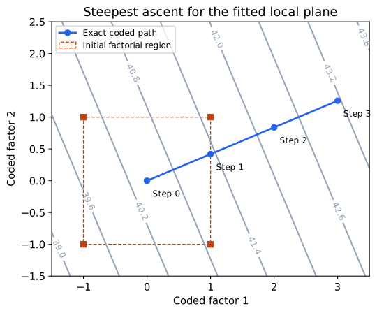
Parallel contours of the fitted local plane and an exact steepest-ascent path perpendicular to them.

The visual shows the geometry of the fitted plane, not measured responses away from the initial design. Its straight contours do not validate long-range extrapolation.

Walk, Observe, and Recenter¶

At each new setting, collect a response. Continue only while the improvement remains useful and the conditions remain feasible. A decline can suggest that the best region along that path has been passed, but one low observation can also be noise or a time effect.

Consider replicate or confirmation runs when variability could change the decision.
Keep track of drift and batch changes during the sequential experiment.
If several factors are constrained, choose a feasible direction rather than following an infeasible gradient.
If curvature or important interaction is already apparent locally, a plane may be the wrong model for deciding the next direction.

For illustration, ten rounded steps of $(5,2)$ from $(35,155)$ reach $(85,175)$ . Ten exact gradient-ratio steps reach approximately $(85,175.968)$ . Do not mix the rounded natural settings with the exact coded path.

A promising point is not automatically the global optimum. Build a new experiment around it to learn the local response shape.

Recode Around a New Center¶

If a promising region is around $(85,175)$ and new low/high levels are $(80,90)$ for A and $(170,180)$ for B, define

x_1^{\mathrm{new}}=\frac{A-85}{5},\qquad x_2^{\mathrm{new}}=\frac{B-175}{5}.

(17)

The old and new coded variables are different coordinates. Reusing the old formula would mislabel the new runs.

Centering alone does not guarantee orthogonality; the actual allocation and replication of the new settings determine the design matrix. A balanced factorial around the new center provides the familiar orthogonal main-effect columns.

Near a stationary region, first-order slopes may become small and curvature matters more. Estimating a full quadratic model requires additional locations that separate the squared-factor columns; repeated common-center runs alone do not do that.