Quadratic Response Surfaces - The Statistics Notebook

A first-order model supplies a direction of improvement. Near an optimum, curvature becomes essential: we need to estimate how the slope changes as each factor moves. A second-order response surface supplies this local shape and a candidate operating point.

At a Glance¶

Locate

Classify & confirm

Set the fitted gradient to zero and solve for the stationary point.

Why More Design Points Are Needed¶

For $k$ quantitative factors, the full quadratic model is

y=\beta_0+\sum_{j=1}^k\beta_jx_j+\sum_{j=1}^k\beta_{jj}x_j^2+\sum_{i<j}\beta_{ij}x_ix_j+\epsilon.

(1)

There are $p=1+2k+k(k-1)/2=(k+1)(k+2)/2$ coefficients, including the intercept. Estimating them requires a design matrix of rank $p$ , not merely $p$ observations.

At two-level factorial corners, every $x_j^2=1$ . Thus all pure quadratic columns coincide with the intercept. Adding the center separates the intercept from the sum of the quadratic coefficients, but the quadratic columns still coincide with one another. Opposing curvatures can even cancel in that sum.

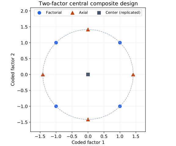
Axial points vary one factor while holding the others at zero. They provide the information needed to separate individual quadratic terms.

Central Composite Designs¶

A central composite design (CCD) combines three sets of runs:

Component	Coded settings	Number of runs without replication outside the center
Factorial	All combinations of $x_j=\pm1$	$2^k$
Axial	One coordinate $\pm\alpha$ , all others zero	$2k$
Center	All coordinates zero	$n_C$

The total is $N=2^k+2k+n_C$ . For $k\geq2$ and distinct axial settings, there are $2^k+2k+1$ distinct conditions. Repeated center runs add pure-error information without adding new locations. A suitable fractional factorial core can reduce the run count, provided the required quadratic model remains estimable.

Choosing the Axial Distance¶

Choice	Meaning	Practical implication
$\alpha=1$	Face-centered CCD	Three levels per factor; axial settings stay within the factorial bounds.
$\alpha=\sqrt{k}$	Spherical geometry	All noncenter points lie at the same radius.
$\alpha=n_F^{1/4}$	Rotatable standard CCD, with an appropriate factorial core and one run per axial point	Prediction variance depends on distance from the center rather than direction.

Spherical geometry and rotatability are different properties. For a full factorial core with $k=2$ , both give $\alpha=\sqrt2$ ; with $k=3$ , they give $\sqrt3$ and $8^{1/4}$ respectively. Replication patterns affect the rotatability condition. See the CCD design guidance for the standard construction.

A face-centered CCD equals the full three-level factorial when $k=2$ , but not generally: with three factors it has 15 distinct settings, versus 27 for a full three-level factorial.

Factorial, axial, and center points in a two-factor CCD

Matrix Form & the Stationary Point¶

Write the fitted surface as

\widehat y(\mathbf x)=\widehat\beta_0+\mathbf b^\mathsf T\mathbf x+\mathbf x^\mathsf T B\mathbf x.

(2)

The vector $\mathbf b$ contains linear coefficients. The symmetric matrix $B$ has pure quadratic coefficients on its diagonal and half each interaction coefficient off the diagonal. With two factors,

B=\begin{pmatrix}\widehat\beta_{11}&\widehat\beta_{12}/2\\\widehat\beta_{12}/2&\widehat\beta_{22}\end{pmatrix}.

(3)

The halving matters because the matrix product contains both $B_{12}x_1x_2$ and $B_{21}x_2x_1$ .

The gradient and Hessian are

\nabla\widehat y=\mathbf b+2B\mathbf x,\qquad H=2B.

(4)

If $B$ is invertible, setting the gradient to zero gives

\boxed{\mathbf x_s=-\tfrac12 B^{-1}\mathbf b}.

(5)

In computation, solve $B\mathbf x_s=-\mathbf b/2$ directly rather than explicitly forming an inverse.

Classifying the Surface¶

Eigenvalues of $B$	Classification
All negative	Strict maximum of the fitted quadratic
All positive	Strict minimum of the fitted quadratic
Both positive and negative	Saddle point
One or more zero	Flat direction; investigate rank and the gradient before claiming an isolated optimum

Negative diagonal entries alone do not guarantee a maximum: a strong interaction can create an upward direction. Eigenvalues check every direction simultaneously.

Worked Optimization¶

Suppose the fitted local surface, using $x_1=(A-85)/5$ and $x_2=(B_{\mathrm{natural}}-175)/5$ , is

\widehat y=79.94+0.995x_1+0.515x_2-1.376x_1^2-1.001x_2^2+0.25x_1x_2.

(10)

Here the curvature matrix is $B=\begin{pmatrix}-1.376&0.125\\0.125&-1.001\end{pmatrix}$ . The matrix symbol $B$ is separate from the natural-unit factor name.

Calculation summary

Quantity	Result
Coded stationary point	$(0.3893,0.3059)$
Natural settings	$(86.947,176.529)$
Curvature eigenvalues	$-1.4138,-0.9632$
Predicted response	80.212

Both eigenvalues are negative, so the fitted stationary point is a local maximum. Feasibility and model adequacy still need checking.

The candidate is approximately $(86.95,176.53)$ in natural units, with predicted response 80.21. Both eigenvalues are negative, so the fitted surface has a maximum there. This is a model prediction, not a new observed outcome.

Adequacy, Constraints & Confirmation¶

A full-rank quadratic fit needs more than algebraic solvability. Check residuals, constant variance, influential runs, and lack of fit. With $g$ distinct conditions and $N$ runs, pure-error df are $N-g$ , residual df are $N-p$ , and lack-of-fit df are $g-p$ . When both components have positive df,

F_{\mathrm{LOF}}=\frac{SS_{\mathrm{LOF}}/(g-p)}{SS_{\mathrm{PE}}/(N-g)}.

(11)

For a two-factor CCD with four corners, four axial points, and five centers, $N=13$ , $g=9$ , $p=6$ : residual df 7 split into 4 pure-error and 3 lack-of-fit df.

A stationary point outside the studied or feasible region is an extrapolation. Optimize within the actual constraints and inspect boundaries if needed. Near-singular curvature can make the calculated location very unstable. Round settings to achievable values, recompute the prediction there, and perform independent confirmation runs.

Sequential augmentation is useful: add axial runs after a factorial-and-center experiment reveals curvature. If stages occur on different days, include stage effects where estimable and check their confounding with curvature; shared center runs help assess stage shifts.