Robust Parameter Design - The Statistics Notebook

A process can hit its target on average yet vary too much in everyday use. Robust parameter design selects controllable settings that give a desirable mean and reduce sensitivity to conditions that vary during operation.

At a Glance¶

Mean response

Response variability

Use the fitted mean model to reach the target response.

Control Factors & Noise Factors¶

Control factors $\mathbf x$ can be set in routine operation, such as pressure or line speed. Noise factors $\mathbf z$ vary in use, such as humidity or incoming material composition. A noise factor may still be deliberately varied during a laboratory experiment.

A crossed array runs outer-array noise settings at each inner-array control setting. A combined array puts both kinds of factors into one experiment. Both can study robustness; the combined approach directly models control-by-noise interactions and can use fewer runs. Choose the design to protect the effects needed for mean and variance prediction.

If a noise factor cannot be manipulated, measured variation may still inform a model, but causal interpretation and coverage of operating conditions require extra care.

From One Model to Mean & Variance¶

For two controls and one noise factor, consider

y=\beta_0+\beta_1x_1+\beta_2x_2+\beta_{12}x_1x_2+\gamma z+\delta_1x_1z+\delta_2x_2z+\epsilon.

(1)

Group terms as

y=f(\mathbf x)+g(\mathbf x)z+\epsilon,

(2)

where $f=\beta_0+\beta_1x_1+\beta_2x_2+\beta_{12}x_1x_2$ and $g=\gamma+\delta_1x_1+\delta_2x_2$ . The function $g$ is sensitivity to the noise factor.

Assume the operating distribution has $E[z]=0$ , $\operatorname{Var}(z)=\sigma_z^2$ , and residual error has mean zero, variance $\sigma^2$ , and zero covariance with $z$ . Holding controls fixed,

\boxed{m(\mathbf x)=E[y\mid\mathbf x]=f(\mathbf x)},

(3)

\boxed{v(\mathbf x)=\operatorname{Var}(y\mid\mathbf x)=g(\mathbf x)^2\sigma_z^2+\sigma^2}.

(4)

These models contain only controls, so they can be optimized before the future noise value is known.

Coding experimental levels as $-1,+1$ does not establish that the operating variance of $z$ is one. Supply that variance from a defensible operating distribution or choose a standardization that makes it one. If $E[z]=\mu_z\ne0$ , the mean becomes $f+g\mu_z$ .

For several noise factors, write $y=f+\mathbf g^\mathsf T\mathbf z+\epsilon$ . With centered noise and covariance matrix $\Sigma_z$ ,

v(\mathbf x)=\mathbf g(\mathbf x)^\mathsf T\Sigma_z\mathbf g(\mathbf x)+\sigma^2.

(6)

Correlation between noise factors contributes cross terms. If quadratic noise terms are included in the response model, their expectations need not vanish; derive the moments again rather than dropping every noise-containing term.

Define the Objective Before Optimizing¶

For a target $T$ , one option is to minimize $v(\mathbf x)$ subject to $m(\mathbf x)=T$ and feasible control bounds. Another is expected squared target error:

E[(y-T)^2\mid\mathbf x]=v(\mathbf x)+[m(\mathbf x)-T]^2.

(7)

This explicitly balances spread and bias. If no control-by-noise interaction is present and residual variance is constant, this model offers no control setting that changes variance. That means there is no variance-reduction opportunity within this fitted model, not that the process is automatically insensitive to noise.

Worked Bottle-Filling Example¶

Let the response be deviation from nominal fill height, so the target is zero.

Factor	Role	Low	High
Carbonation	Noise $z$	10%	20%
Pressure	Control $x_B$	25 PSI	30 PSI
Line speed	Control $x_C$	200/min	250/min

A reduced fitted model is

\widehat y=1+1.125x_B+0.875x_C+1.5z+0.375x_Bz,

(8)

with residual standard deviation $s=0.8118$ on 11 df. Under centered noise with $\sigma_z^2=1$ ,

\widehat m=1+1.125x_B+0.875x_C,\qquad \widehat v=(1.5+0.375x_B)^2+0.8118^2.

(9)

On $-1\leq x_B\leq1$ , the sensitivity $1.5+0.375x_B$ is positive and increasing. Its square is therefore minimized at $x_B=-1$ . This choice can also meet the mean target:

0=1-1.125+0.875x_C\quad\Longrightarrow\quad x_C=\frac17.

(10)

Decoding gives pressure $27.5+2.5(-1)=25$ PSI and speed $225+25/7\approx228.57$ bottles/min.

Calculation summary

Quantity	Result
Pressure	25 PSI
Speed	228.571 bottles/min
Predicted variance	1.9246
Predicted standard deviation	1.3873

At coded pressures $-1,0,1$ , predicted variances are respectively $1.9246,2.9090,4.1746$ .

Target mean and changing variance across pressure settings

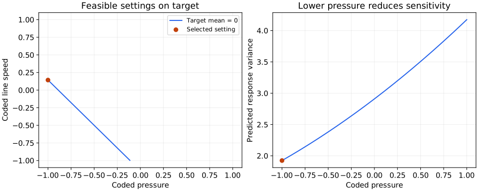
The unconstrained sensitivity-zero setting would be $x_B=-4$ , well outside the studied region. It is not justified by this experiment. At feasible settings, noise still contributes variance: robustness here means reducing that contribution, not eliminating it.

Interpreting & Checking the Recommendation¶

Control-by-noise interaction is useful information: it tells us how to change sensitivity. Preserve model hierarchy when retaining interactions, and assess model adequacy rather than automatically deleting every term with a large p-value.

The variance calculation includes residual variation and assumed operating noise variation, but not uncertainty in the estimated coefficients. Check the recommendation over plausible noise distributions, use confirmation runs across representative noise conditions, and compare both the observed average and spread with predictions. A rounded speed of 229/min changes the coded control and the predicted mean slightly; evaluate the rounded setting explicitly.