Boosting

Boosting

Combines many weak classifiers (that are slightly better than random guessing) to produce one powerful committee.

• Weak classifiers included in the final model do not have equal weights.

AdaBoost¶

• Adaboost is one of the first boosting model with binary targets, $(-1,1)$.

• Fit a weak classifier, $G_m(x)$ on weighted data, then increase weights on misclassified points so that the next round focuses on them.

Process¶

1. Initailize weights, $w_i=\frac{1}{N}, i=1, ...N$

2. For $m_1$ to $M$:
   a. Fit a classifier $G_m(x)$ to the training data using weights $w_i$.
   b. Compute

   $$\mathrm{err}_m \;=\; \frac{\sum_{i=1}^{N} w_i \, I\!\big(y_i \neq G_m(x_i)\big)}{\sum_{i=1}^{N} w_i}$$

   (3)

• This is the weighted fraction of incorrectly classified observations.

  c. Compute

  $$\alpha_m \;=\; \log\!\left(\frac{1-\mathrm{err}_m}{\mathrm{err}_m}\right)$$

  (4)

  d. Set

  $$w_i \leftarrow w_i \exp\!\left[\alpha_m \, I\!\big(y_i \neq G_m(x_i)\big)\right]$$

  (5)

3. Final classification:

   $$G(x) \;=\; \operatorname{sign}\!\left(\sum_{m=1}^{M} \alpha_m \, G_m(x)\right)$$

   (6)

• If classification is done correctly, the weight of an observation does not change.

• If classification is done incorrectly, the weight is increased by multiplying with $\exp{(\alpha_m)}$.

  • $\alpha$ varies with the degree of misclassification.

  • $\alpha$ is large if the error is small.

Normalizing the observation weights¶

After the example’s update, four observations have weight $1/6$ and two have weight $1/3$. Their total is $4/3$. Dividing by this total gives weights $1/8$ for each correct observation and $1/4$ for each incorrect observation. The two mistakes now carry half the total weight.

Only relative weights matter when the next weighted error divides by their sum. Under normalization, correctly classified observations lose relative weight even though their unnormalized weights were unchanged.

For $0<\mathrm{err}_m<1/2$, the learner gets a positive vote. At $1/2$ its vote is zero. A zero error requires a stopping rule because the log ratio diverges. Repeatedly upweighting mistakes can also focus on mislabeled observations; boosting does not automatically distinguish label noise from a difficult but useful case.

Forward Stagewise Additive Modeling¶

• Generally, boosting fits an additive model. Unlike Adaboost, it is not limited to 2-class classification.

• The formula above is a re-written Adaboost classifier.

Estimation¶

• A loss function has to be minimized:

• For example, if we set squared error loss as the loss function,

  $$\min_{\{\beta_m, \gamma_m\}_1^M} \sum_{i=1}^{N} \left(y_i - \sum_{m=1}^{M} \beta_m b(x; \gamma_m)\right)^2$$

  (15)

• In each iteration, we find the best fit to the residual from the previous iteration.

Loss Function

How wrong are we to predict $f_{m-1}(x_i) + \beta_m b(x_i;\gamma_m)$ when the truth is $y_i$?

MART Process¶

1. Initialize $f_0(x) = 0$

2. For $m=1$ to $M$ (total number of iterations),
   Add to the existing model such that the loss function is minimized.

   a. Minimize the loss $\sum^{N}_{i=1}L[y_i, f_{m-1}(x_i) + \beta_mb(x_i;\gamma_m)]$.
   b. Update the function $f_m = f_{m-1}(x) + \beta_mb(x;\gamma_m)$.

• $b(x;\gamma_m)$: The new weak learner fitted this round.

• $\beta_m$: Learning rate or step size for $m$.

• $\gamma_m$: The parameters of the new weak learner.

Logit Boost¶

Logit Boost

A boosting algorithm that uses deviance (log likelihood) as the loss function instead of the exponential loss used in AdaBoost. Outputs a probability between $0, 1$ instead of class labels as in AdaBoost.

• Forward stagewise algoirthm requires an estimate $f_{m-1}(x_i)$.

• Loss function used is the deviance (negative binomial likelihood).

  $$\log L = \sum_{i=1}^{N} \left[ y_i \log p_i + (1 - y_i) \log(1 - p_i) \right]$$

  (16)

• First, derive $p$ as an expression of $f(x)$.

• Rewrite the log likelihood:

• $y$ is coded as $0,1$.

• Ultimately,

  $$f_m \sim f_{m-1}(x_i)+\beta_mb(x_i;\gamma_m)$$

  (19)

MART¶

Multiple Additive Regression Trees

Gradient boosting where weak learners are decision trees specifically.

Assuming that trees ($b(x_i;\gamma_m)$) are being used as weak learners,

1. Initialize $f_0$

2. Fir $m_1$ to $M$:
   a. Compute pseudo residuals.
   b. Fit a regression tree (with $J$ terminal nodes) to pseudo residuals.
   c. For each terminal node, compute fitted values.
   d. Update $f_m=f_{m-1} + \text{ fitted values}$.

3. Output $f_m$ as estimate of $f$.

• Loss function is minimized by going in the opposite direction of the gradient.

  $$r_{im} = -\left[-\frac{\partial l(y_i, f(x_i))}{\partial f(x_i)}\right]_{f = f_{m-1}}$$

  (21)

Residuals depend on the loss¶

For loss $L(y,f)$, the pseudo-residual is

With half-squared error, $L=(y-f)^2/2$, this is the ordinary residual $y-f$. With binary log loss and $f$ measured in log-odds, it is $y-p$. The new tree is a regression tree fitted to these numerical residuals even when the original target is a class label.

The example uses residuals to choose regions, then a Newton approximation for each region’s update:

This combines the first derivative with the curvature of the loss. Classical LogitBoost uses a weighted least-squares Newton procedure; the residual-tree construction here describes gradient tree boosting with Newton leaf updates.

Learning rate and stopping¶

Shrink the update by a learning rate $0<\eta\leq1$:

A smaller $\eta$ takes smaller steps and generally needs more trees. Tune the learning rate, tree size, and number of rounds together. Early stopping selects the number of rounds using validation loss. The test set should not decide when to stop.

XGBoost¶

XGBoost

Optimized and extended implementation of gradient boosting. Uses both first and second derivatives.

Process¶

1. Initialize a constant score appropriate to the loss. For binary log loss, probability 0.5 corresponds to log-odds score 0.

2. Same as regular MART until fitting a tree with $J$ leaves. Fit a regularized tree with a specifieid depth and allows for pruning.

3. Fitted values are computed differently because of the regularization.

Taylor Series¶

Taylor Series

A way to approximate a function using a polynomial built from the function’s derivates at a point.

• If $f$ is analytic and $x$ lies within the convergence interval, then $f(x)=\sum_{n=0}^{\infty}\frac{f^{(n)}(a)}{n!}(x-a)^n$.

  • A finite-order Taylor approximation needs suitable derivatives and a remainder term; infinitely many derivatives alone do not guarantee that the infinite series equals the function.

1st Order Approximation¶

In order to start approximating, the function $f$ needs to be differentiable at or near $a$.

2nd Order Approximation¶

In order to continue with approximation, $f(a)$ needs to exist (twice differentiable near $a$).

Loss Approximation with Taylor Series¶

Second order Taylor series expansion of the first term in regards to $\sum_{i=1}^{n} l\!\left(y_i;\, f_{m-1}(x_i) + \gamma_{im}\right)$:

This approximates the loss for one observation. Sum over observations and add the regularization terms to obtain the objective.

Gaussian Outcomes¶

• XGBoost is a generalization of standard gradient boosting.

• Gaussian outcomes lead to a squared loss function.

• Any proposed split splits one terminal node into two child nodes.

• To evaluate the proposed split, we concentrate on the parent and child nodes only.

  $$\text{similarity}= \frac{\text{sum of residuals}^2}{\text{number of residuals} + v}$$

  (47)

Split gain from the regularized objective¶

Using the notation above, let $G_j=\sum_{i\in R_j}g_i$ and $H_j=\sum_{i\in R_j}h_i$. The part depending on leaf weight $\gamma_j$ is

The factor $1/2$ follows from the objective written above. Omitting it requires rescaling the complexity penalty as well. The leaf penalty does not change the ranking of candidate splits that all add one leaf, but it does change whether a split is worth keeping.

For half-squared loss, $g_i=f_i-y_i$ and $h_i=1$, giving the residual formula above. For binary log loss on a log-odds score, $g_i=p_i-y_i$ and $h_i=p_i(1-p_i)$. The residual-count formula cannot be reused unchanged for binary classification.

Pruning¶

• $\alpha$ does not affect finding out wich split has the highest gain.

• Build a tree until some stopping criteria has been reached (e.g., maximum depth), and then prune all leaves from the bottom that have a negative $\alpha$-adjusted gain.

  • This is equivalent to pruning all leaves with a gain less than a threshold $\alpha$; a raw gain below $\alpha$ is rejected; an already penalty-adjusted gain is compared with 0.

Engineering Improvements¶

Fewer Split Points¶

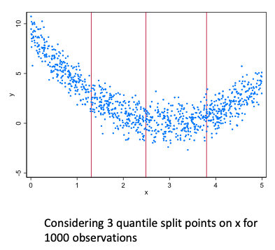
• To determine the best split for a given tree, we need to check every threhold for every variable. (e.g., If 1000 observations, 999 potential splits). This takes a long time. Instead, consider for each variable only quantiles.

Default Missing Value¶

• If there is a missing value, find the split on that $x$-variable as usual on non-missing values.

• Evaluate gain in two options: Add missing values (with non-missing $y$) to the left or the right child node.

• Add missing values to the option leading to the greater gain.

• This is mentioned as sparsity awareness.