k-Nearest Neighbors

• Like the Bayes decision rule, $k$-NN assigns a class using conditional probabilities; it estimates them with local proportions.

  • $k$-NN approximates the conditional probability for a given class with the fraction of observations in local neighborhood of $k$ observations that correspond to the class.

• $k$-NN is a memory based algorithm, so no training is required.

  • $k$-NN does not learn any parameters during training phase; it simply stores the entire training dataset in memory.

  • Unlike neural network or logistic regression, which takes training data and distills it into weights (parameters). Once a model is trained here, we do not need the original data anymore.

  • Neighbor lookup and voting occur at prediction time; the stored data and distance rule together define the model.

• Especially sensitive to variable scaling and standardization.

• Has nonlinear decision boundaries.

  • We do not have to explicitly define what the boundary looks like.

  • Since it votes locally, the boundary naturally bends and curves to follow the actual data structure.

A local vote¶

Suppose the five nearest training observations contain three positives and two negatives. Then $\hat P(Y=1\mid x_0)=3/5=0.6$, and majority voting predicts class 1. The estimate changes when the neighborhood changes; there is no single coefficient vector describing all predictions.

The Bayes classifier also uses a conditional probability at $x_0$. The difference is that it assumes the true probability is known, while $k$-NN estimates it from nearby observations. “No training” means no coefficient-fitting step; choosing a distance, scaling predictors, selecting $k$, and storing the training data are still part of fitting the procedure.

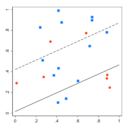
• This is a linear boundary formed by logistic regression; a straight, linear line should seperate data into classes.

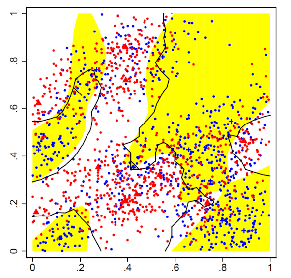
• • From above, yellow lines represent the Bayes classifier, and black lines represent $k$-NN boundaries with ($k=50$).

Bias vs. Variance¶

• Since $k$-NN relies on nearest neighbors to make predictions, 1-NN has low bias but high variance.

  • Conditional probabilities for class assignments are made too locally.

• Increasing $k$ makes the estimate to be more stable (reduce variance.)

• Increasing $k$ also increases the average distance of $k$ training observations to the new point, $x_0$ (increasing bias).

Exceptions¶

• There can be exceptions as when there is a tie between neighboring votes.

• To resolve this:

  • Break ties at random.

  • Increase $k$ until tie is broken.

  • Use 1-NN as a tie breaker (Use the single closest observation.)

Hyperparameter Tuning¶

Choice of $k$¶

• $k$=1 will be very unstable with lots of noise.

• It is better to choose odd number of $k$ to reduce the chance of ties.

• Choose $k$ that yields the smallest validation or cross-validation error.

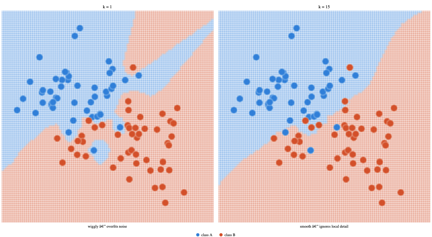
• Small $k$ makes decision boundaries to be very wiggly and twisted. It contorts around every single point, including small clusters of outlier points mixed into the wrong region. Leads to low bias but high variance.

• Large $k$ makes smoother boundary, and largely ignores outlier clusters. They find the overall trend instead. Leads to low variance but higher bias.

Checking the extremes¶

With $k=1$, a training observation usually predicts its own label if it is allowed to be its own neighbor. That near-perfect training accuracy says little about a new observation. For leave-one-out evaluation, exclude the observation being predicted from its candidate neighbors.

At the other extreme, $k=n$ uses the whole training sample for every prediction. The estimated class probabilities are then the overall class proportions, regardless of $x_0$. This is stable but loses local structure.

Choose $k$ on validation folds and then assess the selected value on the test set. An odd $k$ avoids a two-class vote tie, but ties are still possible with three or more classes. Fix the tie-breaking rule in advance so evaluation uses the same prediction rule as future data.

Distance¶

• How are distance among observations calculated?

• Commonly Euclidean distance is used, but there are other metrics.

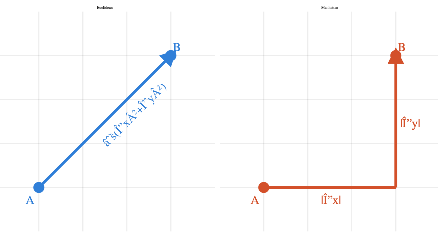
Euclidean Distance¶

• For two points, $(x_1, y_1)$ and $(x_2, y_2)$,

  $$\sqrt{(x_2-x_1)^2+(y_2-y_1)^2}$$

  (3)

• Penalizes large differences in any angle dimension heavily.

• Flying in a straight line, cutting diagonally through buildings as an analogy.

• Useful when:

  • Features are continuous and on similar scales.

  • When we expect diagonal relationships between data.

  • Low to medium dimensionality.

  • Becomes meaningless in high-dimensional data due to the curse of dimensionality, because distances can become concentrated, making near and far points harder to distinguish.

Manhattan Distance¶

• For two points, $(x_1, y_1)$ and $(x_2, y_2)$,

  $$|x_2-x_1| + |y_2-y_1|$$

  (4)

• Also called as the L1.

• Treats each dimension equally and adds up the absolute gap.

• Walk along the grid, only moving horizontally or vertically as an analogy.

• Useful when:

  • Features have been put on comparable scales; Manhattan distance also depends on units.

  • High-dimensional data.

  • Sparse data (like TF-IDF vectors), where most dimensions are zero.

  • Want outliers in one dimension to have less outsized influence.

Similarity¶

• Instead of distance metrics, similarity metric can also be used.

• A decreasing transformation can convert distance to a similarity score, but the reverse transformation need not satisfy all metric properties.

  • Smallest distance goes with greatest similarity.

• Cosine similarity is often used in text mining and document retrieval, because the $X$-matrix is very sparse.

Derivations¶

Nearest Neighbor with Caliper¶

• Used for sparse data where nearest $k$ observations may be far away.

• Isntead of specifying a fixed number of $k$ neighbors, one can use all observations in a caliper (fixed distance) around a new observation.

• Could be risky if there are no observations in a given caliper leading to missing values.

Weighted neighbors and sparse neighborhoods¶

A closer observation can receive more weight:

For example, inverse-distance weights give nearby points more influence. Exact duplicates need a separate rule because dividing by a distance of zero is undefined. Weighting is another modeling choice to validate, rather than an automatic improvement.

As the number of relevant dimensions grows, finding observations close in all coordinates requires much more data. Irrelevant coordinates can make the problem worse by dominating distance without contributing useful information about the class. Standardization addresses units, but it does not identify which variables matter.

A fixed $k$ expands the neighborhood in sparse regions. A fixed-radius caliper instead keeps locality but may have few or no neighbors. In that case, an explicit “insufficient nearby data” rule is more informative than quietly assigning a confident class.