Random Forest

Bootstrap¶

Bootstrap

A resampling technique where you repeatedly sample from your own data with replacement to estimate properties of a statistic.

• Samples contain the same number of observations as the original sample.

• Often used to compute empirical standard errors.

Bagging¶

• Stands for Boostrap Aggregation.

• To reduce variance of a model by training many versions of it on different boostrap samples and averaging their predictions.

• Most suitable to be used for models that have high variance.

  • Trees have high variance because single trees are very unstable.

  • Logistic regression has low variance.

Regression¶

• For $i=1,...B$, draw a boostrap sample $i$, and learn and predict on the bootstrapped sample. Then average the results.

Classification¶

There are two ways to apply bagging to classification.

1. Use majority vote.

2. Average the proportions from the individual classifiers and choose the class with the greatest average proportion.

• The bagged predictor is the class with the largest average proportion:

• $\hat{f}_k(x)$ is the average proportion for the class $k$.

• $p_b$ is the proportion in the corresponding terminal leaf for bag $b$.

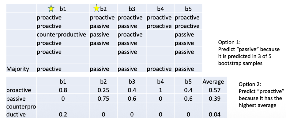
• Two levels of aggregation:

  1. Observations within each leaf. Each leaf contains multiple training observations and predicts the majority class among them.

  2. Observations across trees. Each tree votes to the class for the new observation. The final prediction is the majority vote across all $B$ trees.

Random Forest¶

• Takes bagging as a precursor.

• Comparison to Trees:

  • Trees: For each split, find the best split among $p$ variables.

  • Random Forest: For each new split, choose a different random subset.

Process¶

1. For $b=1$ to $B$, draw a bootstrap sample. From each split, select $m$ out of $p$ variables at random. Choose the best variable/split among $m$ variables.

• This randmonness is what splits random forest from bagging.

2. Output the ensembled trees.

3. Make predictions.

• Prediction for regression: Average prediction values over all trees.

• Prediction for classification: Majority vote.

Tuning Parameters¶

• Standard error of an average decreases with square root of the number of summands. (Number of trees)

  $$se(\bar{Y}) = \frac{1}{\sqrt n}se(Y_i)$$

  (4)

Why randomizing features helps¶

The $1/\sqrt{B}$ reduction applies to independent predictions with equal variance. Trees trained from the same dataset are correlated. If each tree prediction has variance $\sigma^2$ and every pair has correlation $\rho$, then

As $B$ grows, the second term vanishes, but the shared component remains. Bagging averages unstable trees; random feature subsets also try to reduce their correlation. Otherwise, one strong predictor may be chosen near the top of almost every tree.

Reducing $m$ can decorrelate trees while making individual trees weaker. This is why choosing $m$ involves a tradeoff. Adding more trees mainly reduces the randomness of the ensemble average; it does not fix poor features or an unsuitable validation scheme. Validation error may fluctuate as trees are added, even when the ensemble is approaching a stable limit.

Out of Bag Samples¶

Out-of-bag (OOB)

Samples in training datat which didn’t get picked when a bootstrap sample was created for a tree in a Random Forest.

• In general, each bootstrap sample on avearge uses about $\frac{2}{3}$ of their observations and leave the rest unused due to its inherent sampling with replacement.

• The probability of not selecting 1 of $n$ observations $n$ times in a row:

Making an OOB prediction¶

The probability above approaches $e^{-1}\approx0.368$. A bootstrap sample has $n$ draws but only about $0.632n$ distinct observations on average. Duplicates account for the difference.

For observation $i$, collect predictions only from trees whose bootstrap samples excluded $i$. Aggregate those predictions, compare with $y_i$, and repeat for every training observation. Each observation is evaluated by a different subset of trees.

OOB error is a useful internal estimate when observations are independent and representative. It does not solve leakage from repeated subjects or time ordering. Also, repeatedly choosing settings to improve OOB error makes it part of model selection; an independent final evaluation still has a separate role.

Permutation

Shuffling values of a column across rows. This keeps the same values, but breaks the relationship with target.

Variable Importance¶

• Exactl how $x$-variables are related to the outcome is unclear; black-box model.

Check with OOB¶

1. For a given tree, compute OOB prediction accuracy (Using observations not used in tree construction.)

2. For a variable $j$, randomly permute the values in the OOB sample (Destroy all prediction power variable $j$ might have had.)

3. Decrease in prediction accuracy is due to variable $j$.

4. Average this decrease over all trees and use as a measure of importance.

Usage and Limitation¶

Reading importance scores¶

Permutation importance asks how much predictive performance worsens when one feature’s information is disrupted. It does not measure the effect of intervening on that feature.

If two predictors contain similar information, the model may still predict well after one is shuffled. Conversely, shuffling one predictor can create combinations that were rare or absent in the original data. Correlated predictors therefore need care when interpreting the scores.

A different measure, impurity importance, adds up the training impurity reductions assigned to each predictor. Predictors with many possible split points can receive high scores partly because they offered more chances to improve training fit. The two importance measures answer different questions and need not rank variables the same way.