Logistic Regression

The linear predictor can take any real value, while a probability must stay between 0 and 1. A link function connects these two scales.

Linearity¶

The equations below define the link and convert the linear predictor back to a probability.

\text{logit}(p) = \log\frac{p}{1-p}

(1)

\text{logit}(p) = \beta_0 + \beta_1x_1 + ... + \beta_px_p

(2)

Log-odds (logit) allow transformation from range $(0,1)$ to $(-\infty, \infty)$ .
Hence, $\text{logit}(p)$ outputs a number on the entire real line.
$p = \frac{e^{\beta_0+\beta_1x}}{1+e^{\beta_0+\beta_1x}}$
(3)

$p = \text{expit}(\beta_0+\beta_1x)$
(4)

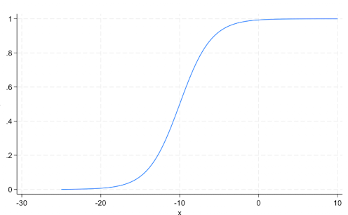
Classifying a new observation $i$ :
$\hat{y_i} = \begin{cases} 1 & \text{if } p_i \geq 0.5 \space \text{(Or any threshold)}\\ 0 & \text{otherwise} \end{cases}$
(5)

Odds¶

\operatorname{odds}=\frac{p}{1-p}=\frac{P(Y=1\mid X)}{P(Y=0\mid X)}

(6)

Interpreting Coefficients¶

Assume that the two equations below differ by 1 unit of $x_i$ .

\text{log}\frac{p_i}{1-p_i} = \beta_0 + \beta_1(x_1+1) + ... + \beta_p x_p

(7)

\text{log}\frac{p_j}{1-p_j} = \beta_0 + \beta_1x_1 + ... + \beta_p x_p

(8)

And,

\text{log}\frac{p_i}{1-p_i} - \text{log}\frac{p_j}{1-p_j} = \beta_1

(9)

\text{log}\frac{\frac{p_i}{1-p_i}}{\frac{p_j}{1-p_j}}= \beta_1

(10)

\beta_1 = \text{log}\frac{\text{odds}_i}{\text{odds}_j}

(11)

\text{exp}(\beta_1) = \frac{\text{odds}_i}{\text{odds}_j}

(12)

We can rearrange it as,

\text{odds}_j \times \text{exp}(\beta_1) = \text{odds}_i

(13)

We can state that increasing $x_i$ by 1, the odds of $y=1$ increase by factor of $\exp(\beta_1)$ .

Odds are not probabilities¶

An odds ratio multiplies the odds, not the probability. If $p=0.2$ , the odds are $0.2/0.8=0.25$ . Doubling those odds gives 0.5, so the new probability is $0.5/(1+0.5)=1/3$ , not 0.4.

For a change of $\Delta$ units in $x_j$ , the odds ratio is $e^{\beta_j\Delta}$ , holding the other predictors fixed. This interpretation assumes that $x_j$ enters without interactions or nonlinear terms. With an interaction, its effect also depends on the interacting variable.

For a simple linear predictor, the probability slope is

\frac{\partial p}{\partial x_j}=\beta_jp(1-p).

(14)

The same coefficient therefore produces different probability changes at different starting probabilities. The intercept gives the log-odds when all predictors are zero; that baseline may be outside the observed data unless the predictors have been centered.

Example

Understanding Coefficients¶

\text{logit}(p_\text{admit}) = -10 + 0.15x_{\text{Average}}

(15)

Assume that the equation above depicts the probability of being admitted to graudate school as a function of the applicant’s undergrad average, where an example value of $x$ would be $75, 80$ .

Here, we can interpret that each additional percentage point on the average score increases the odds of admission by a factor of $\text{exp}(0.15) = 1.16$ .

In logistic regression, unpenalized coefficient estimates are approximately normally distributed in large samples under regularity conditions. Thus, it follows a $z$ -statistic, where $z = \frac{\hat{\beta} - \beta_0}{se}$ . If $\hat{\beta}$ is approximately normal, then $z \sim N(0,1)$ .

Interpreting Probability¶

Assume that if $x=80$ , our equation would be:

\text{logit}(p_\text{admit}) = -10 + 0.15 \times 80 = 2

(16)

And since We know that:

p = \frac{1}{1+e^{-z}} \space \text{where} \space z=2

(17)

p = \frac{1}{1+e^{-2}} \approx 0.8808

(18)

We can conclude that when $x=80$ , the model predicts that the probability of admission is approximately 88.08%.

Estimation¶

L(\beta) = \prod_{i=1}^N \left[p(x_i;\beta)\right]^{y_i} \cdot \left[1 - p(x_i;\beta)\right]^{1 - y_i}

(19)

The likelihood is maximized over the coefficients by Maximum Likelihood, where $p(x; \beta) = \frac{e^{x'\beta}}{1+e^{x'\beta}}$ , and where $y_i$ is 0 or 1, and $x_i$ is a vector.

Properties of MLE¶

Property	Meaning
Consistency	Under regularity conditions, estimates converge to the true parameter as the sample size grows: $\hat\beta\to\beta$ .
Asymptotic normality	In large samples, the estimator has an approximately normal sampling distribution under regularity conditions.
Efficiency	MLE is asymptotically efficient under regularity conditions; this is not a universal finite-sample guarantee.
Invariance	If $\hat\theta$ is an MLE of $\theta$ , then $g(\hat\theta)$ is an MLE of $g(\theta)$ .

An unbiased estimator satisfies $E[\hat\theta]=\theta$ : across repeated samples, its average equals the true parameter. This is a separate property; an MLE need not be unbiased in a finite sample.

From likelihood to loss¶

Each observation contributes $p_i$ if $y_i=1$ and $1-p_i$ if $y_i=0$ . Taking logs turns the product into

\ell(\beta)=\sum_{i=1}^n\{y_i\log p_i+(1-y_i)\log(1-p_i)\}.

(20)

Maximizing this expression is equivalent to minimizing log loss, $-\ell(\beta)/n$ . A confident wrong prediction receives a large penalty. Predicting $p=0.01$ for an observation with $y=1$ contributes $-\log(0.01)\approx4.61$ , compared with $-\log(0.5)\approx0.69$ at $p=0.5$ .

Separation¶

If a predictor or combination of predictors perfectly separates the classes, increasingly large coefficients can keep improving the unpenalized likelihood. A finite MLE may not exist. Large standard errors and extreme fitted probabilities can be symptoms of this problem.

Regularization limits coefficient growth. It is also useful with many correlated predictors. Approximate normal inference for the unpenalized MLE needs a sufficiently informative sample and regularity conditions; it is not an exact finite-sample result.

Usage

Logistic regression is less prone to overfitting.
- Due to linearity making the fit highly inflexible, with no penalty tuning parameter in the unregularized formulation.
- Cannot bend or wiggle to fit noise.
- With only raw predictors, captures a linear log-odds relationship; derived features and interactions allow richer patterns.
Excels at explaining how individual variables relate to the outcome.
Use for binary outcomes and if we want to capture probabilities.
Suggested dataset size is approximately medium.
Simple, stable, and well-regularized. Hence performs well on real classification problems.
Has low variance, so does not overfit easily.
- Since logistic regression models ( $\log(\frac{p}{1-p})$ ) are linear in features, and the decision boundary cannot adapt too much to random noise. Cannot bend to fit small fluctuations.
Can produce useful probability estimates when the model is appropriate; calibration should still be checked.

Limitations

When the data relationship is highly nonlinear, with complex interactions and nonlinear boundaries.
- Instead, explore gradient boosting or random forest.
High-dimensional sparse data needs regularization; regularized logistic regression can work well in this setting.
When classes are extremely imbalanced.
- Can still use logistic regression, but needs a proper class weighing and threshold tuning.
- This is because the model is trained to minimize log loss, not to treat both classes equally.
- When there is a class majorly dominating the other, logistic regression model can predict everything as major class and still achieve higher accuracy.
- Class weighing assigns higher penalty to mistakes on minority class.

School Notes

Solutions Key

LASSO Regression¶

Regularization¶

Criterion¶

Criterion: MSE + Penalty.
- Least squares estimator: $\text{MSE} = \frac{\text{RSS}}{n}$ , where RSS is the Residual Sum Squares, and is $\text{RSS} = \sum_{i=1}^n(y_i-\beta^tx)^2$ .
- The Least Square Estimator finds the coefficients that minimize the sum of squared errors between observed and predicted values.
- Hence, $\text{Criterion} = \frac{\text{RSS}}{n} + \text{Penalty}$ for Least Squares Estimator.

L2 Ridge Regression¶

L2 penalty is defined as:

\text{Criterion} = \frac{\text{RSS}}{n} + \frac{1}{n}\|\beta \|^2\text{,} \space \text{where } \| \beta \| = \sqrt{\sum_{i=1}^p\beta_i^2}

(21)

$\| \beta \|$ is the L2 or Euclidean norm of coefficients.
This penalty favours smaller squared coefficients; strongly penalizes large coefficients.
No penalty when all coefficients equal zero.
Dividing by $n$ can be skipped.
Can be simplified to:
$\text{Criterion} = \frac{\text{RSS}}{n} + \frac{1}{n}\sum_{j=1}^p{\beta_j^2}$
(22)
- Ridge uses the squared L2 norm from the start. Removing a square root from only the penalty would change the objective and generally its minimizer.
With regularization parameter $\lambda$ that decides on how large a penalty should be,
$\text{Criterion} = \frac{\text{RSS}}{n} + \frac{\lambda}{n}\sum_{j=1}^p{\beta_j^2}\text{ ; }\lambda> 0$
(23)
Coefficients do not shrink to zero. When variables are highly correlated, L2 regulazation performs better.

Methods for the best $\lambda$ ¶

Estimate $\lambda$ via cross validation.
Find the $\beta$ ’s in the linear model that minimize the criterion above.
Rely on AIC or BIC.

Different Notation¶

Can also be written as...

\min_{\beta}\text{RSS} \quad \text{such that} \quad \sum_{j=1}^p \beta_j^2 \le s

(24)

Here, errors are minimized subject to a constraint.

$s$ : constraint on total coefficient size.
For every $\lambda$ , there exists some $s$ .
For every $s$ , there exists some $\lambda$ .
If there are two $x$ -variables, then $\beta_1^2+\beta_2^2 \leq s$ .

L1 LASSO Regression¶

When we don’t want to penalize large coefficients as strongly.

\text{Criterion} = \frac{\text{RSS}}{n} + \frac{\lambda}{n}\sum_{j=1}^p{|\beta_j|}\text{ ; }\lambda> 0

(25)

Here, coefficients are shrinked to zero. Used for variable selection.
Whether lasso or ridge predicts better depends on the data; compare them using validation error.
Large $\lambda$ means selecting fewer variables.

Different Notation¶

\min_{\beta}\text{RSS} \quad \text{such that} \quad \sum_{j=1}^p |\beta_j| \le s

(26)

$s$ : constraint on total coefficient size.
If there are two $x$ -variables, then $|\beta_1|+|\beta_2| \leq s$ .

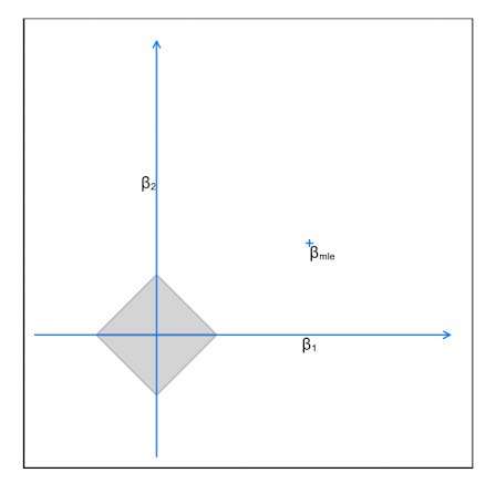
Every corners of the diamond correspond to one of $\beta_1$ and $\beta_2$ being 0.

Property	L1 (Lasso)	L2 (Ridge)
Penalty	$\sum \lvert\beta_j\rvert$	$\sum \beta_j^2$
Feature selection	Yes (sets some coefficients to 0)	No (keeps all features)
Sparsity	Produces sparse models	No sparsity
Correlated features	Tends to pick one	Distributes weights across them
Stability	Less stable	More stable
Best use case	High-dimensional, few relevant vars	Many relevant, correlated features
Interpretability	High	Moderate

Regularized Logistic Regression¶

From the regularization criterion above, replace $\text{RSS}$ with $\log \text{likelihood}$ .
- Instead of RSS minimization, likelihood must be maximized. (Or, minimize the negative likelihood.)

\text{Criterion} = -\log\text{likelihood} + \frac{\lambda}{n}\sum_{j=1}^p{\beta_j^2}\text{ ; }\lambda> 0

(27)

\text{Criterion} = -\log\text{likelihood} + \frac{\lambda}{n}\sum_{j=1}^p{\beta_j^2}\cdot\text{Var}(x_j)

(28)

Sometimes, $\text{Var}(x_j)$ is included by taking into account the different scales of $x$ -variables.
- Because, if left as is, $\beta_j^2$ assigns smaller coefficient to features with large scales. To make this fair across all features, apply variance-weighted penalty.
- In this case, no need to standardize $x$ -variables.

Keeping the penalty convention consistent¶

A convenient convention is average negative log-likelihood plus a penalty:

\min_{\beta_0,\beta}\left[-\frac{\ell(\beta_0,\beta)}{n}+\lambda P(\beta)\right],

(29)

where $P(\beta)=\sum_j|\beta_j|$ for lasso and $P(\beta)=\tfrac12\sum_j\beta_j^2$ for ridge. The intercept is usually left unpenalized. Factors such as $n$ and $1/2$ change the numerical meaning of $\lambda$ , so compare formulas before comparing penalty values.

Standardize continuous predictors before applying a common penalty. Otherwise, changing a variable from metres to centimetres changes the coefficient size and therefore its penalty, even though the underlying information is unchanged. Choose $\lambda$ using validation data or cross-validation, with scaling estimated within each training fold.

Lasso can set coefficients exactly to zero; ridge usually shrinks them continuously. Neither gives a universal prediction advantage. With correlated predictors, several different lasso selections may give similar predictions, so selection alone should not be treated as evidence that one variable is uniquely important.

SVM Regularization¶

SVM tries to maximize the margin between classes while allowing some errors ( $\epsilon_i$ ).
SVM is another regularized optimization problem with a different loss function.
- Loss function: Measure of how wrong the model’s predictions are. Smaller the better.
- $\text{Loss = error between } y \text{ and } \hat{y}$ .
Find a boundary, $f(x) = \beta_0 + \beta^T x$ , that can make correct classifications with a large margin.
$\min_{\beta} \sum_{i=1}^n \max(0, 1 - y_i f(x_i)) + \lambda \sum_{j=1}^p \beta_j^2$
(30)
We are minimizng the loss and penalty added together.
- Loss: $\sum_{i=1}^n \max(0, 1 - y_i f(x_i))$ . This is hinge loss.
- $y_i \in \{-1, +1\}$ ; True label classes are either encoded as -1 or +1.
- In SVM, +1 refers to one class, and -1 refers to other class.

Case	Value
Correct and far away	0
Correct but close	small penalty
Wrong	large penalty

Solutions Key

Linearity¶

Odds¶

Interpreting Coefficients¶

Odds are not probabilities¶

Estimation¶

Properties of MLE¶

From likelihood to loss¶

Separation¶

LASSO Regression¶

Regularization¶

Criterion¶

L2 Ridge Regression¶

Methods for the best λ\lambdaλ¶

Different Notation¶

L1 LASSO Regression¶

Different Notation¶

Regularized Logistic Regression¶

Keeping the penalty convention consistent¶

SVM Regularization¶

Methods for the best $\lambda$ ¶