SVM: Linear

Support Vector Machine

A classification algorithm that finds the best boundary to separate two classes ($-1,1$) by maximizing the distance to the closest observations.

• Observations that are included within the dashed lines are called as support vectors.

• Observations below the hyperplane are classified as $y=(-1)$.

• Observations above the hyperplane are classified as $y=(+1)$.

• Since $y$ is either $\{-1, 1\}$, $y(\beta_0 + \beta_1x_1 + ... \beta_px_p)$ is positive for correctly classified observations, negative for misclassified observations, and zero on the boundary.

• For every correctly classified observation, this statement holds: $y(\beta_0 + \beta_1x_1 + ... \beta_px_p) \geq 0$.

  • This can be redefined with a margin, $M$, such that: $y(\beta_0 + \beta_1x_1 + ... \beta_px_p) \geq M$.

  • $M$ is the distance of the line to the closest observation.

Linearly Separable¶

Maximum Margin Classifier¶

• $y(\beta_0 + \beta_1x_1 + ... \beta_px_p) \geq M$ implies no errors.

• $\max_{\beta_0,\beta_1,\ldots,\beta_p,\; M}$ implies to find the hyperplane that gives the largest possible margin $M$ between the two classes.

  • These coefficients, $\beta$, should give the largerst possible margin $M$.

  • Noramlization of $\beta$ controls the margin width.

Normalization

Fixing the scale of the $\beta$ vector so that it has a specific length.

$$\| \beta \| = \sqrt{\beta^2_1+\beta^2_2+...+\beta^2_p}$$

(6)

• By notating $\sum_{j=1}^{p} \beta_j^{2} = 1$, the coefficient scale is fixed to 1. Can also be written as $\|\beta\| = 1$.

• Ensure that the constraint on $\beta$ is met by dividing by the norm.

This proves that when you normalize $\beta$, the result has length 1.

• $\beta$ can be multiplied by any positive constant, $c$, because both sides will scale equally. The actual values of $\beta$ don’t uniquely matter, only their ratios do.

Formula Rearrangements¶

• This is the original form that maximizes margin $M$, while keeping $\beta$ a unit vector. It is hard to optimize because of the $\|\beta\|=1$ constraint.

• Subject to: “Under the condition that...” Hence, Find the $\beta$ that makes $\|\beta^2\|$ as small as possible, but only consider solutions where every training point is correctly classified with margin $\geq 1$.

• Maimizing $M$ is the same thing as minimizing $\frac{1}{M}$.

• Drop the $\|\beta\|$ constraint. Absorb the unit norm constraitn into the inequality, and $\beta$ can be any scale.

• If we assume $M=\frac{1}{\|\beta\|}$,

  $$\min_{\beta_j, j=1,\ldots,p} \|\beta\|^2 \quad \text{subject to} \quad y_i(\beta_0 + x_i^T\beta) \geq 1$$

  (14)

• Minimizing $\|\beta\|$ is the same thing as minimizing $\|\beta\|^2$. If $\|\beta\|$ is minimized at some $\|\beta*\|$, then $\|\beta\|^2$ is also minimized at the exact point at $\beta*$.

• Final optimization for quadratic optimization problem with a linear constant:

  $$\min_{\beta_j, j=1,\ldots,p} \frac{1}{2}\|\beta\|^2 \quad \text{subject to} \quad y_i(\beta_0 + x_i^T\beta) \geq 1$$

  (15)

Geometric margin and coefficient scale¶

Multiplying both $\beta_0$ and $\beta$ by the same positive constant does not change the separating hyperplane. The geometric distance of $x_i$ from it is

In the unit-norm formulation, the signed score is already a signed distance. In the canonical formulation, the closest correctly classified points satisfy $y_i(\beta_0+x_i^T\beta)=1$, so the distance to either margin plane is $1/\|\beta\|$. The full width between the two margin planes is $2/\|\beta\|$.

This normalization is why minimizing $\|\beta\|^2/2$ maximizes the margin. The intercept is optimized too, but it is not included in the norm: shifting the plane does not change the length of its normal vector.

• To minimizie $\|\beta\|^2$ as a constraint, the Lagragian trick merges the objective and constraint into a single expression.

  $$L = \frac{1}{2}\|\beta\|^2 - \sum_{i=1}^{N} \alpha_i\left[y_i(\beta_0 + x_i^T\beta) - 1\right]$$

  (17)

• Set derivatives with respect to $\beta_j, \beta_o$ to zero (to find a minimum of a function):

• Writing $\beta$ in vector notation avoiding index $j$:

• Thus, we know $\beta$ is a linear combination of the observations.

Lagrange Multiplier

A variable that convers a constrained optimization problem into an unconstriained one.

$$L = f(x) - \alpha \cdot g(x)$$

(23)

$$f(x) = \text{Function to minimize}, g(x) = \text{constraint}, \alpha = \text{Lagrange multiplier}$$

(24)

$\alpha$ measures how much the constraint is pushing back against the objective. The larger $\alpha$ is, more influeential the constraint is.

• In the hard-margin formulation, only observations on a margin plane can have $\alpha_i>0$.

• Observations strictly beyond the margin planes have $\alpha_i=0$.

Kuhn-Tucker Condition

Rules that the optimal solution must satisfy when you have an optimization problem with inequality constraints.

To optimize $\max_xf(x)$, $\text{subject to } g(x) \leq 0$,

If $x*$ is a local optimum, subject to regularity conditions, then there exist a constant multiplier $\alpha_i$ such that,

$$g(x*) \leq 0$$

(25)

$$\alpha_i \geq 0$$

(26)

$$\alpha_i \cdot g(x*) = 0 \qquad \forall i$$

(27)

Complementary Slackness¶

• Stemming from $\alpha_i \cdot g(x*) = 0$, complementary so that the two terms complement each other to make zero. At least one factor must be zero; both can be zero.

• A point $x_i$ is on the boundary if $\big[\, y_i(\beta_0 + x_i^{\top}\beta) - 1 \,\big] = 0$.

• Also, if $\alpha_i > 0$, then $x_i$ is on the boundary. If $x_i$ is not on the boundary, then $a_i = 0$.

Beta Optimization¶

Hence, this proves that estimation of $\beta$ is only dependent on support vectors.

Not Linearly Separable¶

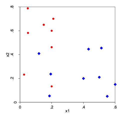
• In cases like this, two classes are not completely separable.

• Non-linearly separable classess can be managed with some errors. This is the slack variables, or $\epsilon_i$.

• All observations between the margin, and the separating hyperplane, and all misclassified observations (on the other side of the separating hyperplane) have a positive $\epsilon_i > 0$.

• Errors, $\epsilon_i$, of the correctly classified observations before the margin is 0.

Error Limit¶

• The sum of $\epsilon_i$ cannot exceed $C$.

• $C$ is the tuning parameter; the cost parameter.

  • Larger $C$ value allows for more error and have larger margins. Also correspond to more support vectors because more observations lie within the larger margins.

Two meanings of $C$¶

Above, $C$ is a budget in $\sum_i\epsilon_i\leq C$. Increasing that budget permits more total margin violation. Another common formulation uses $C$ as a penalty coefficient:

Here, larger $C$ makes violations more expensive, so its direction is opposite to the budget convention. Always check the objective before interpreting the tuning parameter.

For the smallest feasible slack, $\xi_i=\max(0,1-y_if(x_i))$:

• $\xi_i=0$: on or beyond the correct margin plane.

• $0<\xi_i<1$: correctly classified but inside the margin.

• $\xi_i=1$: on the decision boundary.

• $\xi_i>1$: misclassified.

In this penalty formulation, the dual coefficients satisfy $0\leq\alpha_i\leq C$. A point with $0<\alpha_i<C$ lies on a margin plane; points inside the margin can have $\alpha_i=C$. Support vectors therefore need not all lie exactly on the margin in a soft-margin model.

Prediction¶

• How a new observation is being classified is decided by which side of the hyperplane the observation falls on.

• Mathematically, the sign of the estimated value, $\text{sign}(\hat{f(x)})$, determines whether the observation is classified as +1 or -1, where:

• where $<.. , ..>$ is the inner dot product, $\hat{\alpha_i} > 0, i=1,...n$ is the estimated coefficients arising during optimization.

  $$K(x, x_i) = \sum_{j=1}^p x_jx_{ij}$$

  (37)

• The dot product is a similarity measure affected by both direction and magnitude, where $x_i$ is an observation from training data and $x$ is an observation from test data.

SVM: Kernels¶

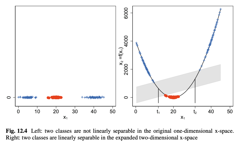
• Add quadratic derived variables, so that the linear separation becomes possible in an expanded space, but it is still nonlinear in the original space.

• In the original space (Assume we have $x_1, x_2$), classes may not be separable.

• Add new features like $x_1^2, x_2^2, x_1x_2$ and now we’re in the high dimensional, expanded space. In this space, a linear boundary may separate patterns that could not be separated in the original coordinates.

• But when you project that boundary back to the original space, it looks nonlinear.

• Adding nonlinearities in $x$.

• The original feature space has $p$ variables, but expanded feature spaces have $2*p$ variables.

• SVM is a linear method in the expanded features space.

• SVM accommodates nonlinearity in the original feature space.

Kernels

A function that computes the similarity between two points in a higher dimensional space, without actually going there. Instead of expanding to high dimensions (which can be slow), directly computes what the dot product in that high dimensional space would have been.

$$K(x_i, x_j) = \langle \phi(x_i), \phi(x_j) \rangle$$

(39)

$$\text{where } \phi = \text{ transformation to high dimensions.}$$

(40)

• How kernels expand feature space is not obvious.

Predictions¶

• From $\hat{\beta} = \sum_{i \in S} \hat{a_i}y_ix_u$, the predicted value is:

Can be re-written as:

The solution depends only on the inner product of the observations, not on the observations themselves.

Non-Linear Expansion¶

• Rather than adding quadratic terms to the $x$-variables, it is possible to expand the feature space as a function of the original $x$-variables.

Linear Kernel¶

• Referes to the standard SVM without any additional $x$-variables.

• Has no additonal tuning parameters.

• Often preferred in text mining applications with $n$-gram variables.

  • Sparse matrices and indicator variables.

Polynomial Kernel¶

• Tuning parameters: $\beta_0, \gamma_0, d \space (d > 0)$.

  • In practice, often set $\beta_0 = 0, d = 2 \text{ or } 3 \text{ and tune } \gamma \text{ and } C$

RBF Kernel¶

• Also called as Gaussian Kernel.

  $$K(x_i, x_{i'}) = \exp\!\left( -\gamma \sum_{j=1}^{p} \left(x_{ij} - x_{i'j}\right)^2 \right)$$

  (57)

• Tuning parameter: $\gamma > 0$.

  • $\gamma$ determines how fast the influence of neighboring observations on the classification of the test observation drops off as a function of distance. Larger $\gamma$ leads to a local fit.

• $xi'$ is a test observation.

• When a test observation is very far from training observation, the kernel value approaches 0 as the exponent becomes increasingly negative.

  • Training observations far from test observation contribute very little to classification.

• Most popular choice.

• Corresponds to an infinite number of $x$-variables.

Interpreting $\gamma$ together with $C$¶

For the RBF kernel, two observations a distance $d$ apart have similarity $e^{-\gamma d^2}$. At $d=0$, it is 1; as distance grows, the kernel value approaches 0. Larger $\gamma$ makes each observation’s influence more local.

A large $\gamma$ and a large penalty-form $C$ can give a highly irregular boundary. A small $\gamma$ makes similarities vary more slowly, but its effect still depends on $C$ and the scaled distances. Tune them together using validation folds, fitting the scaling transformation within each fold.

A nonlinear feature map makes more boundaries available; it does not guarantee that every dataset becomes separable. Two observations with identical predictors and opposite labels remain indistinguishable under any deterministic feature map.

Sigmoid Kernel¶

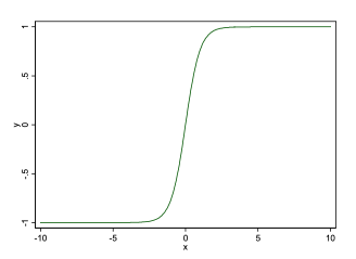
• Tuning parameters: $\gamma > 0, \beta$.

• Not commonly used because of some undesirable theoretical properties.

Platt’s Method¶

Platt Scaling

A method to convert SVM’s raw decision scores into probabilities.

• Since logistic regression computes a probability which is rounded up or down for classification, SVM yield a score.

  • Positive scores: the uncalibrated decision rule predicts $y=+1$.

  • Negative scores: the uncalibrated decision rule predicts $y=-1$.

    $$\text{score} = \hat{f}(x) = \hat{\beta_0} + \sum_{i \in S} \hat{\alpha_i}y_iK(x, x_i)$$

    (60)

Converting Scores into Probabilities¶

• This is Platt’s way of estimating probabilities based on the score.

• If a probability is needed, we can use logistic regression on the score:

  $$\log \frac{p}{1-p} = \beta_0 + \beta_1 \hat{f}(x)$$

  (61)

• The probabilities can be estimated as usual by solving for $p$.

Fitting the calibration step¶

The decision score gives a side of the boundary and a margin-related magnitude. A score of 2 does not mean a probability of 0.88 unless a particular fitted calibration map makes it so.

Fit the sigmoid mapping using held-out scores or out-of-fold predictions, then evaluate it on separate data. Fitting the map to the same in-sample scores used to train the SVM can make probability estimates too optimistic. Calibration can improve the meaning of probabilities without changing the underlying ordering when the fitted map is increasing.

Multi-Class SVM¶

• Typically, SVM only allows for two classes.

• Can extend two-class classifiers:

1. One vs. All¶

• More common.

• With $K$ classes, apply SVM once for each class.

  • Class $k$ vs. all remaining claases.

• Each SVM classifier gives a score $f(x)$ for class $k$ (vs. all others.)

• Predict the class $k$ that has the highest score $f(x)$.

2. One vs. One¶

• $k$ classes give ($k$ choose 2) possible pairs.

• SVM is conducted on each pair.

• Keep track of which class wins each time.

• Predict the class with the most wins.